The Jacobian Matrix: Introducing Vector Calculus

We learn how to construct and apply a matrix of partial derivatives known as the Jacobian matrix. In the process, we also introduce vector calculus.

The Jacobian matrix is a matrix containing the first-order partial derivatives of a function. It gives us the slope of the function along multiple dimensions.

Previously, we’ve discussed how to take the partial derivative of a function with several variables. We can differentiate the function with respect to each variable while keeping the remaining variables constant. Remember that the derivative is nothing but the slope of a function at a particular point. If we take the multivariate function

f(x, y) = x^2 + 3y

The derivative with respect to one variable x will give us the slope along the x dimension.

\frac{\partial{f(x,y)}}{\partial{x}} = 2x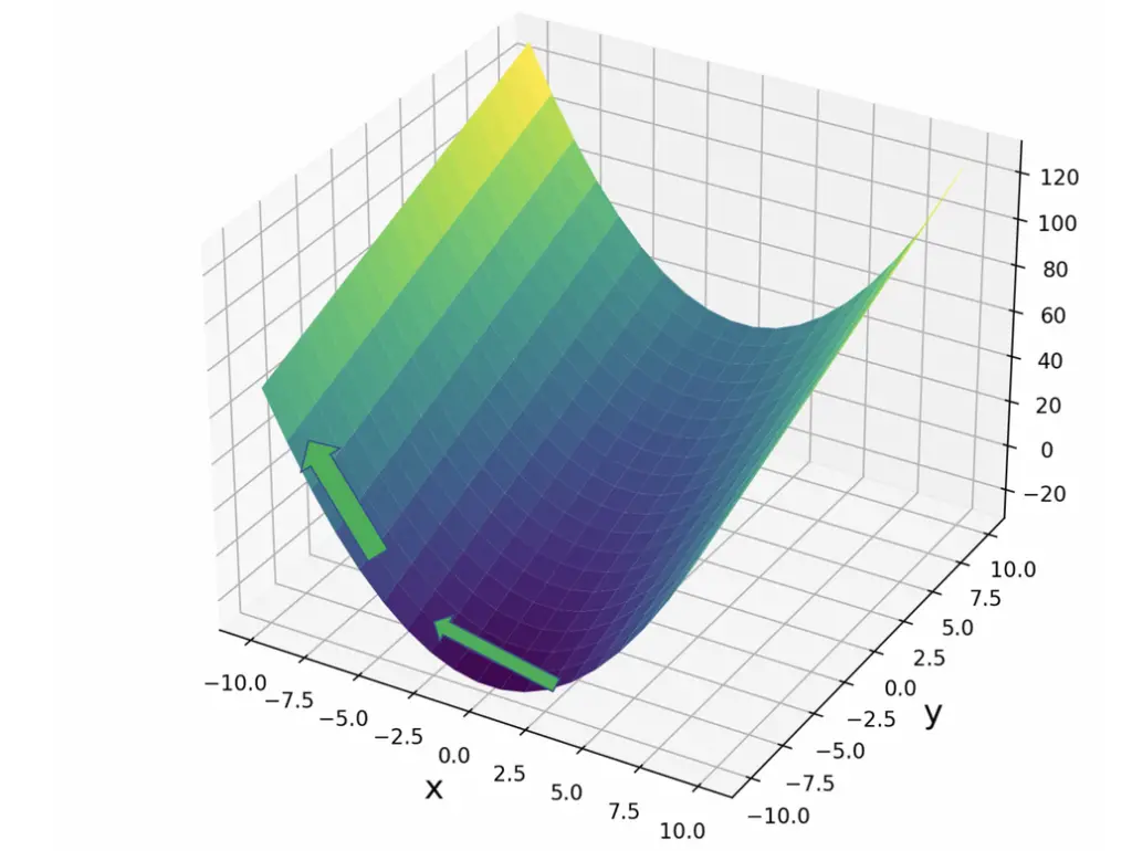

Since x^2 is an exponential term, the slope becomes steeper as we move away from the origin.

Taking the partial derivative with respect to y gives us the slope along the y dimension.

\frac{\partial{f(x,y)}}{\partial{y}} = 3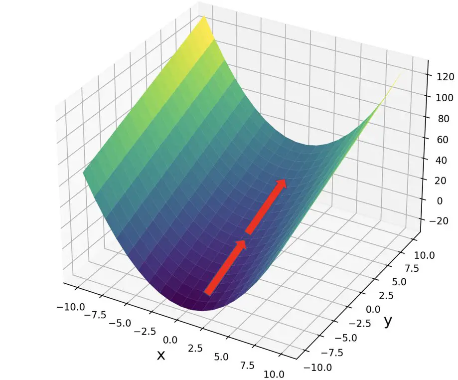

3y is a linear term, therefore the slope along the y axis remains constant.

Gradient Definition: Jacobian Row Vector

What about the total derivative with respect to x and y? Since we are differentiating with respect to x and y, it is the slope along both dimensions.
We can express this as a row vector.

df(x,y) =  
\begin{bmatrix}
    \frac{\partial{f(x,y)}}{\partial{x}} & 
     \frac{\partial{f(x,y)}}{\partial{y}}
  \end{bmatrix}

This is known as the Jacobian matrix. In this simple case with a scalar-valued function, the Jacobian is a vector of partial derivatives with respect to the variables of that function. The length of the vector is equivalent to the number of independent variables in the function.

In our particular example, we can easily “assemble” the Jacobian since we already calculated the partial derivatives.

df(x,y) =  
\begin{bmatrix}
    2x &
    3
  \end{bmatrix}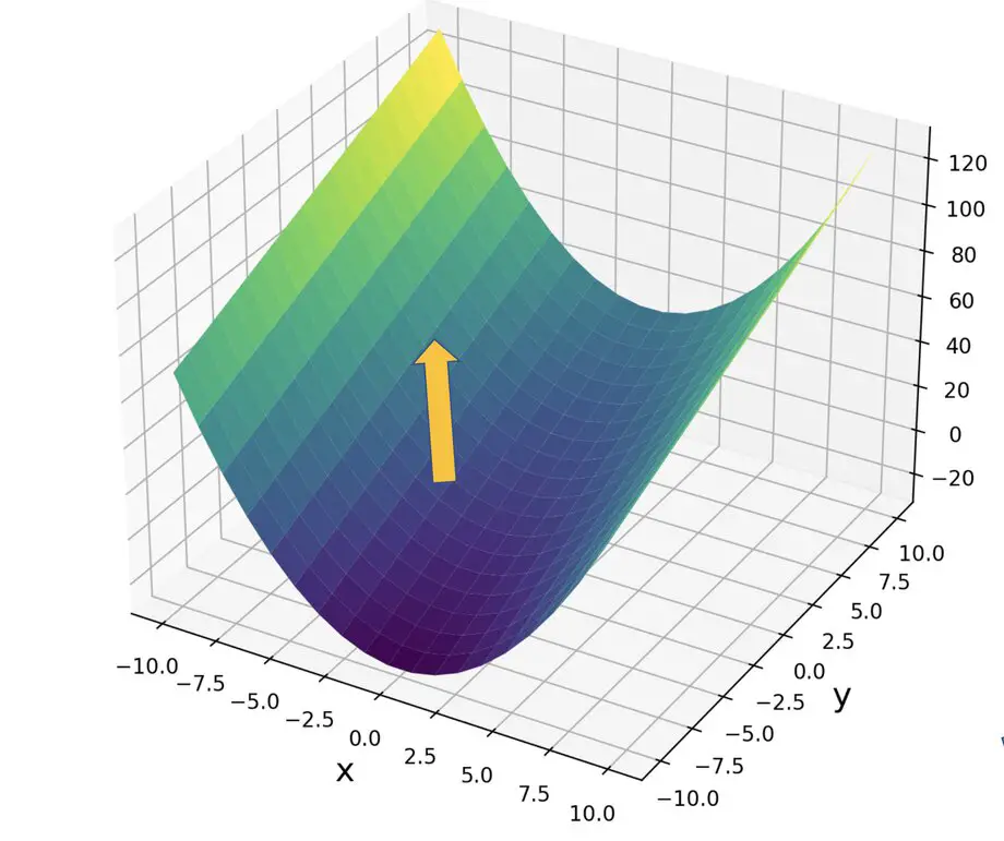

As you’ll hopefully see, the Jacobian can be expressed as a vector. The vector points in the direction of the greatest slope, while its magnitude is proportional to the steepness of the slope at that particular point. This is also known as the gradient of a function. Remember that, unless you are dealing with linear functions and constant slopes, the Jacobian will differ from point to point. To be precise, we’d have to say that the Jacobian is the best linear approximation of the true gradient at a specific point.

Note: if you are unfamiliar with vectors and matrices or need a refresher, I’d suggest checking out my series on linear algebra for machine learning.

Jacobian Matrix

As we’ve seen, the Jacobian of a function of real numbers is a vector. We can expand the definition of the Jacobian to vector-valued functions.

f(x) = 
\begin{bmatrix}
  f_1(x) \\
  ...\\
  f_m(x)
  \end{bmatrix}

Our function vector has m entries. The resulting Jacobian will be an m \times n matrix, where n is the number of partial derivatives. Each row m in the matrix contains the partial derivatives corresponding to the equivalent row m in the function vector.

\frac{df(x)}{dx} = 
\begin{bmatrix}
  \frac{\partial f_1(x)}{\partial x_1} & ... & \frac{\partial f_1(x)}{\partial x_n} \\

  ...\\
  \frac{\partial f_m(x)}{\partial x_1} & ... &   \frac{\partial f_m(x)}{\partial x_n}
  \end{bmatrix}

What’s the use of the Jacobian?

We can use the Jacobian matrix to transform from one vector space to another. Furthermore, if the matrix is square, we can obtain the determinant. The value of the Jacobian determinant gives us the factor by which the area or volume described by our function changes when we perform the transformation. Confused? Let’s do an example to make this clearer.

We take our standard vector space spanned by the vectors x and y

x =\begin{bmatrix}
   1 \\
  0
  \end{bmatrix}\;
y =\begin{bmatrix}
   0 \\
  1
  \end{bmatrix}

Assume we have another vector space spanned by u and v, where u and v are functions of x and y

u = 3x - y\\
v = x - 2y

Now our Jacobian matrix J can be obtained.

J = 
\begin{bmatrix}
  \frac{\partial u}{\partial x} & \frac{\partial u}{\partial y} \\

  \frac{\partial v}{\partial x} &    \frac{\partial v}{\partial y}
  \end{bmatrix}

= 
\begin{bmatrix}
  3 & -1 \\
  1 &    -2
  \end{bmatrix}

If you want to transform any vector from the xy vector space to the uv vector space, You multiply by the Jacobian.
You might say: “This is easy. You only took the coefficients of the functions u and v, and put them in a matrix.”

These are just linear functions. Accordingly, the gradient expressed by the Jacobian will remain constant. No calculus is necessary here. But if you are dealing with non-linear transformations, the pure linear algebra approach isn’t enough anymore. The Jacobian itself will not only contain constants because the transformation will differ from point to point.

We can still calculate the value of the determinant.

det(J) = 3 \times (-2) - (-1) \times (1) = -5

This gives us the factor by which an area is scaled when transforming from the xy to the uv space. Again, here we are dealing with a constant because functions describing the transformations are linear.

Summary

The Jacobian points us in the direction of the highest local point. In the next post, we learn about the Hessian matrix, which helps us determine whether that point constitutes a global maximum.

This post is part of a series on Calculus for Machine Learning. To read the other posts, go to the index.