The Fourier Transform and Its Math Explained From Scratch

In this post we will build the mathematical knowledge for understanding the Fourier Transform from the very foundations. In the first section we will briefly discuss sinusoidal function and complex numbers as they relate to Fourier transforms. Next, we will develop an understanding of Fourier series and how we can approximate periodic functions using sines and cosines. Lastly, we investigate how we can use all the previously introduced concepts to approximate non-periodic functions and to transform them to the frequency domain using the Fourier Transform.

The Fourier transform describes a process of transforming a signal from a representation in the time domain to a representation in the frequency domain. The Fourier transform thus allows us to decompose a signal into its component frequencies. It is applied to a wide variety of fields such as image and sound processing (light and sound signals), signal analysis, and the design of electrical circuits.

Why Do We Perform a Fourier Transformation?

In many areas, such as signal processing and the modeling of dynamic systems, problems are often easier to solve in the frequency domain than in the time domain. The behavior of technical systems and processes is often described by linear differential equations with fixed coefficients. Solving these equations may be very complicated. One of the most compelling reasons for using Fourier Transforms is that translating those problems into the frequency domain makes resolving them easier because we replace non-periodic functions with periodic ones.

Foundations of Fourier Transformations

The fundamental idea behind Fourier transformations is that a function can be expressed as a weighted sum of periodic basis functions such as sines and cosines. In fact, the Fourier transform expresses a signal as a sum of sinusoids which we call “a representation in Fourier space.” Once you’ve transformed a signal into Fourier space using a Fourier transform, you can filter out specific parts of the signal based on the frequency. Then you can transform the signal back into its original space by applying an inverse Fourier transform. When processing sound or images, this is especially useful for filtering noise that would otherwise be hard to detect.

Understanding Sinusoidal Functions

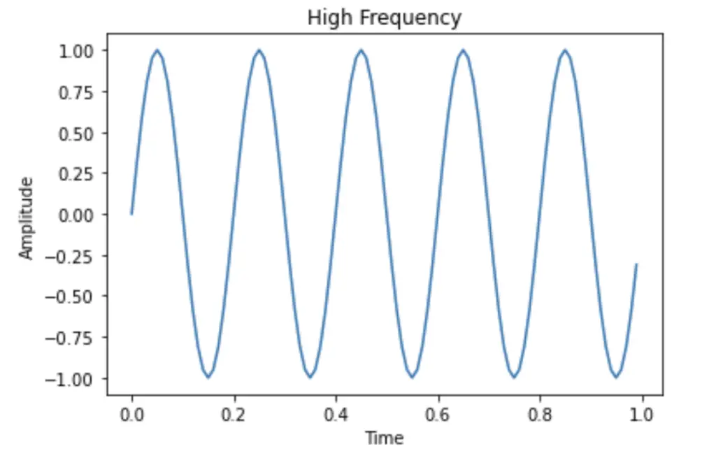
A sinusoid is a common periodic mathematical function used to express frequencies. Sinusoids can be completely described by their period, wavelength, and frequency.

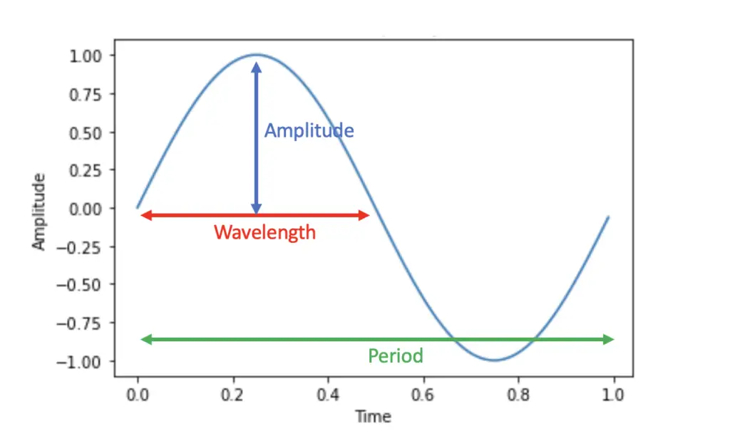
A standard sine wave completes one period (one full cycle) in 2π radians. The basic function describing a sine wave therefore is:

y = sin(2\pi)

In this case, y will equal 0 because the expression sin(2π) gives us the point after one period where y is the amplitude. If we want to calculate a certain point along the sinus function, we need to add the time into the equation. If a full period T lasts one second and we want to find the point along the sinusoid at time t 0.2 seconds, we can add these factors to the sinusoid.

y = sin(\frac{2 \pi  t}{T})

y = sin(\frac{2 \pi  \times0.2}{1})

Instead of the sine, we could equally use the cosine, which would result in a phase shift by π/2 radians.

What is a Frequency?

A frequency expresses the number of occurrences of a repeating event within a certain timeframe. It can be expressed and graphed as a mathematical function.

A frequency of a sinusoid can be calculated by simply taking 1 over the period T (the time it takes for the wave to complete one full cycle).

f = \frac{1}{T}

If the wave needs 1/10 of a second to complete a full cycle, it has a frequency of 10 cycles per second or 10 hertz.

Now we can easily add the frequency into the equation:

y = sin(2 \pi tf)

In practice, we encounter frequencies everywhere where we have signals. For example, a sound frequency is simply a periodic vibration over time that produces a certain pitch.

Complex Numbers and Polar Representation

While Fourier Transforms can be expressed without the use of complex numbers, the expression becomes much more succinct. I’m not going to offer a comprehensive introduction to complex numbers here, but only do a quick recap of the concepts that are necessary for Fourier transforms. For a comprehensive introduction, I highly recommend the free Coursera course Introduction to complex analysis.

A complex number is a number that consists of a real and an imaginary part. The complex number z can be expressed as a sum of a real part (x) and an imaginary part (iy).

z = x + iy

Complex numbers are represented in a coordinate system known as the complex plane, where the real numbers are plotted on the x-axis, and the imaginary numbers are plotted on the y-axis.

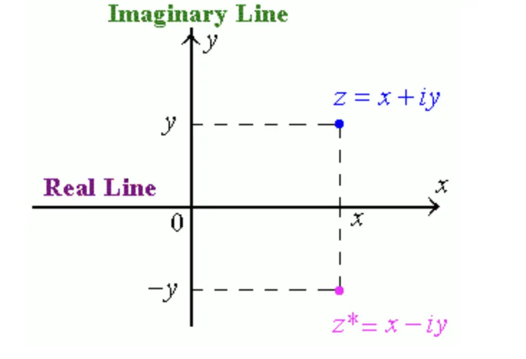
So the complex number z can be expressed as a vector in a 2-dimensional coordinate system.

Adding and Subtracting Complex Numbers

When performing basic operations such as addition and subtraction of complex numbers, you sum or subtract the real and the imaginary parts, respectively.

z_1 + z_2 = (x_1 + x_2) + i(y_1 + y_2)

z_1 - z_2 = (x_1 - x_2) + i(y_1 - y_2)

Magnitude

The magnitude m of a complex number is the square root of the sum of the squares of the real part and the imaginary part.

m = |z| = \sqrt{x^2 +y^2}

Polar Representation

From trigonometry, we know that we can represent the sides of a right-angled triangle as products of an adjacent side and the sine or cosine of an angle θ. This knowledge forms the basis of the polar representation in a complex number plane.

Concretely, we can represent the real component x and the imaginary component y as follows:

x = m \;cos (\theta)

y = m \;sin (\theta)

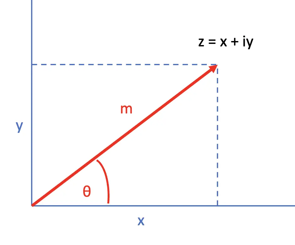
Whith this knowledge, we can represent the complete number z in the polar system.

z=x+iy = m \;cos (\theta) + im \;sin (\theta) =  m[\;cos (\theta) + i \;sin (\theta)]

Euler’s Identity

Euler’s identity states that for any real number θ, the following identity holds:

e^{i\theta} = cos(\theta) + i\;sin(\theta)

Since the angle θ is a real number, we can express the complex number z as a product of the magnitude m and Euler’s number e.

z = m e^{i\theta}

What is a Fourier Series?

Before we move on to Fourier transformations, we need to understand the Fourier series.

The fundamental idea behind the Fourier series is that a periodic function can be described as a sum of sine and cosine waves of different frequencies.

To illustrate the idea, let’s take a periodic function y of time t. The function y is a simple step function with period 2π.

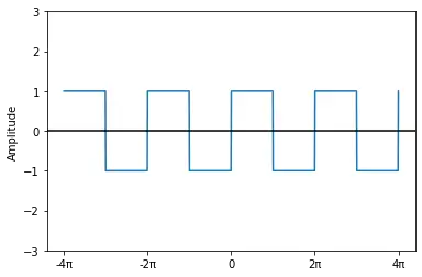
If we naively try to approximate the function through a sine wave and a cosine wave with period 2π, we get the following result (orange is the sine wave, and green is the cosine wave).

y(t) = sin(2\pi) \\
y(t) = cos(2\pi) \\

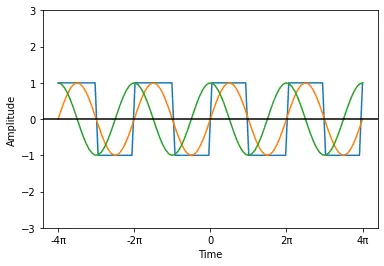
Evidently, the sine wave does a better job at approximating the real y(t) than the cosine wave. But it still isn’t close to the real form of the function. Joseph Fourier had the brilliant insight that we can get arbitrarily close to the real form of the function by adding multiple sines and cosine waves of progressively larger frequencies multiplied by a weighting factor. He expressed it in the Fourier series where a and b are weighting factors, and L is half the period of the function.

y(t) = a_0 + \sum_{n=1} ^N [a_n cos(\frac{n \pi}{L} t) + b_n sin( \frac{n \pi}{L} t)]

Theoretically, you can expand this series for an infinite number of N. The more terms you add in practice, the closer you’ll approximate the original function.

Why does a Fourier Series Approximate Functions?

Fourier further derived that given the period 2L, the weighting factors are equivalent to:

a_0 = \frac{1}{2L}\int^L_{-L} f(t)dt

a_n = \frac{1}{L} \int^L_{-L} f(t) cos(\frac{n \pi}{L} t)dt \;\; for\; n={1,2,3,...}

b_n = \frac{1}{L} \int^L_{-L} f(t) sin(\frac{n \pi}{L} t)dt \;\; for\; n={1,2,3,...}

Since, in our case, the period is equivalent to 2π, we can replace L with π:

L = \pi

Accordingly, our representation of the Fourier series can be simplified:

y(t) = a_0 + \sum_{n=1} ^N [a_n cos(n t) + b_n sin( n t)] 

Not only will this approach find the correct weighting factors. It will shrink or eliminate sinusoids if they are irrelevant or detrimental and magnify those that are relevant at approximating the function. Sine is an odd function, while cosine is an even function. If you try to approximate an even function, the Fourier series should eliminate the sine terms and retain the cosine term and vice versa.

Example: Approximating a Square Wave Using a Fourier Series

To see why this works, let’s calculate some of the weighting factors for our square wave. It is an odd function, so the cosine terms should shrink to 0. The square wave forms alternating blocks that I’ve labeled Q above and below the x-axis. The factor a0 gives us the initial offset from the x-axis. Since the square wave has equal proportions below the x-axis and above the x-axis, we expect a0 to be equal to 0.

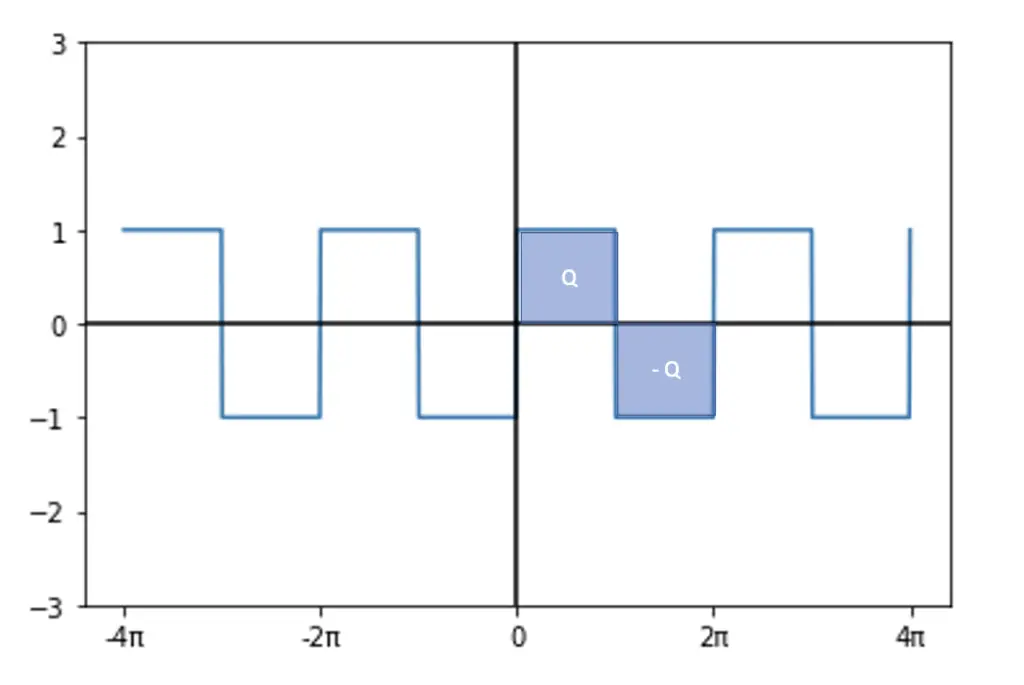
To see whether this is true, let’s take the formula for a0 and calculate the integral over one full period from 0 to 2π. Since the function is periodic, the a0 calculated over one period should be representative of the full function. We split the calculation into two intervals. One ranges from 0 to π and another one from π to 2π. This allows us to precisely capture the areas Q and for -Q formed by the step function. Accordingly, we will use the same split when calculating the approximations.

a_0 = \frac{1}{2\pi}\int^{2 \pi}_{0} f(t)dt =  \frac{1}{2\pi} \left[ \int^{\pi}_{0} f(t)dt  +\int^{2\pi}_{\pi} f(t)dt] \right] 

a_0 = \frac{1}{2\pi} \left[ Q -Q\right] = 0

Note that the integral calculates the area under the curve. So the integral from 0 to π gives us Q, and the integral from π to 2π gives us -Q. We don’t have to do the full calculation to see that Q and -Q will cancel each other out, resulting in 0.

Let’s calculate the first factor a1 for the cosine approximation over the interval from 0 to 2π.

a_1 = \frac{1}{\pi} \int^{2\pi}_{0} f(t) cos(\frac{1 \pi}{\pi} t)dt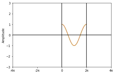

Looking at the plot, we can see that the areas under the curve and above the curve will cancel each other out in the areas from 0 to π and π to 2π. If you resolve the following integrals, you’ll see that they both yield 0.

a_1 = \frac{1}{\pi} \left[ \int^{\pi}_{0} f(t) cos( t)dt +\int^{2\pi}_{\pi} f(t) cos( t)dt \right ]

= \frac{1}{\pi} \left[ 0 + 0  \right ] = 0

Next, we calculate the factor b1 for the sine approximation from 0 to 2π.

b_1 = \frac{1}{\pi} \int^{2\pi}_{0} f(t) sin(\frac{1 \pi}{\pi} t)dt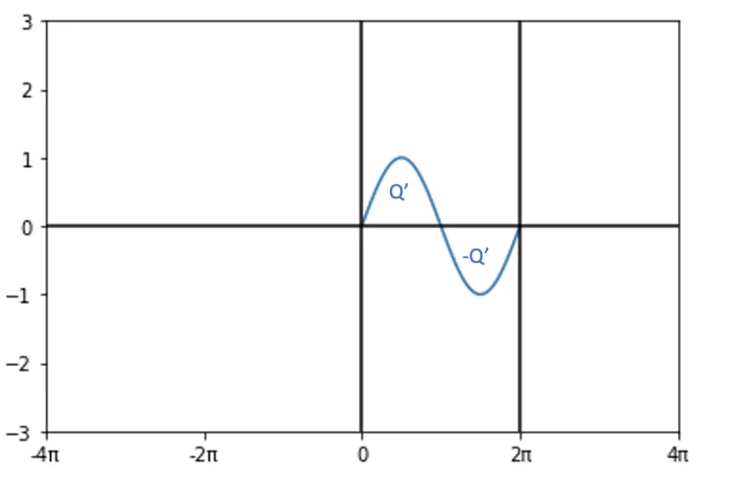 

If we take the integrals again in 2 steps from 0 to π and π to 2π, we get two areas (Q’, and -Q’) that do not cancel each other.

b_1 = \frac{1}{\pi} \left[ \int^{\pi}_{0} Q' sin( t)dt +\int^{2\pi}_{\pi} (-Q')sin( t)dt \right ]

If you evaluate the integrals in these intervals, you should get the following result.

b_1 = 2Q' + 2Q' = \frac{4Q'}{\pi}

As expected and as we’ve seen above in our naive approximation, the cosine terms disappear, and the sine-containing terms are retained because sine does a better job at approximating the function in this case.
You can continue adding terms of increasing frequency to the series, which should get you closer and closer to the actual function.

Here is a little illustration of what the approximation should look like for N=10 and N=50.

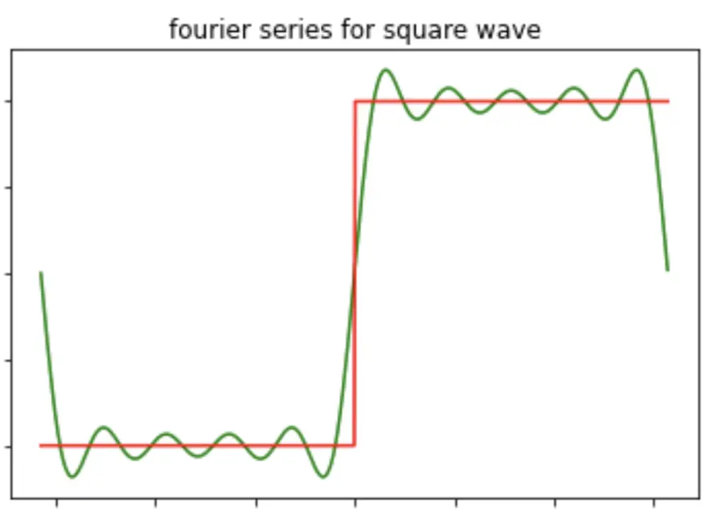
N=10

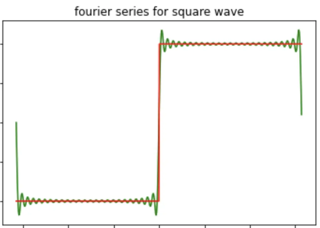
N=50

I won’t continue doing the expansion by hand here, but you are welcome to do so yourself. Here is a great video series that goes through several steps of approximating the square wave. A large part of my explanation is based on this video series.

The Fourier Basis

One of the most mathematical reasons why Fourier transforms work is that the basis functions it relies on (sine and cosine) form an orthogonal basis. Once you’ve projected a function into a new vector basis, you can represent it as a linear combination of the basis vectors. So the Fourier transform is basically a vector projection into the orthogonal basis formed by sine and cosine.

If your memory of vector projections and orthogonal bases is a bit rusty or you don’t understand why this is significant, check out this post on vector projections I wrote (opens in a new tab).

We can show that the Fourier basis is indeed orthogonal by taking our Fourier series with period 2π and showing that the integral over the sum of the basis functions equals zero. In linear algebra, this is equivalent to taking the dot product between two orthogonal vectors, which also equals 0.

f(t)=a_0+\sum_{n=1}^{N}a_n\cos(2\pi nt)+b_n\sin(2\pi nt)

\int_{[0,1]}\cos(2\pi nt)\sin(2\pi mt)dt=0 

If you calculate the integral, you should see that this holds wherever n is not equal to m.

Complex Representation of the Fourier Series

In the previous section, we worked with the Fourier series in the real number domain. With Euler’s identity

e^{int} = cos(nt) + i\;sin(nt)

we can express the Fourier series much more succinctly using complex notation (ignoring the initial factor a_0)

y(t) = \sum_{n=1} ^N [a_n cos(n t) + b_n sin( n t)] 

y(t) = \sum_{n=1} ^N c_n e^{int}

Or if we use our initial expression of the Fourier Series.

y(t) = \sum_{n=1} ^N c_n e^{ in \omega t } \; where \; \omega = \frac{2\pi}{L} 

How Do We Arrive at Coefficient c?

We’ve established before that the basis functions of the Fourier series form an orthogonal basis. Now we’ve managed to summarize the basis function in one complex coefficient. Accordingly, the complex expression e^{ in \omega t } represents a set of orthogonal basis functions.

Much like above, we can prove this by calculating the inner product between e^{ in \omega t } and its complex conjugate e^{ -im \omega t } . It should equal zero for all expressions where t is not equal to m. We integrate over the interval from -T/2 to T/2 because this gives us a nice symmetric expression.

\frac{1}{L} \int^{L/2}_{-L/2} e^{ in \omega t } e^{ -im \omega t } dt = 0 \;where \;m\neq n

If we think about the Fourier series as a vector projection, this orthogonality relationship allows us to express the coefficient c_m as a vector projection of y(t) onto the orthogonal basis vectors contained in e^{ in \omega t } .

c_m = \frac{y(t) e^{ in \omega t } }{e^{ in \omega t } e^{ in \omega t }} 
= \frac{\frac{1}{L} \int^{L/2}_{-L/2} y(t) e^{ -im \omega t } dt}{\frac{1}{L} \int^{L/2}_{-L/2} e^{ im \omega t } e^{ -im \omega t } dt }=  \frac{1}{L} y(t) e^{ -im \omega t } dt

Again, if the concept of vector projections and why this works is unclear, check out the post on vector projections.

I also recommend watching the following video, which offers a more in-depth explanation of the same concepts.

The Continuous Fourier Transform

We’ve done a lot of groundwork in the preceding sections. Getting to the Fourier transform from the Fourier series is now just a small step. The Fourier series can only be used to approximate periodic functions and translate them from the time domain into the frequency domain. But how do we translate non-periodic functions into the frequency domain?

Here is the gist: If we let the period of a periodic function tend towards infinity, we can assume that even an aperiodic function ends at some undefined point and repeats itself. Thus, the function becomes periodic in the limit. Accordingly, we can represent aperiodic functions using a Fourier series with an infinite period. As a consequence, ω becomes an infinitesimally small quantity dω.

L \rightarrow \infty, \;\;w =\frac{2\pi}{L} \;therefore\;w \rightarrow dw

Since the frequency ω becomes infinitesimally small, the discrete frequencies turn into a continuous frequency spectrum. Therefore we need an integral over a period from -\infty, \infty.

The Fourier transform, the transforms a function y(t) from the original domain into the frequency domain can now be expressed as follows:

\hat y(\omega) = F(y(t)) = \int^{\infty}_{-\infty} y(t) e^{-i\omega t} dt

For transforming a function from the frequency domain back to the original domain, we can use the reverse Fourier transform.

y(t) = F^{-1}(\hat y(\omega)) = \frac{1}{2 \pi} \int^{\infty}_{-\infty} \hat y(\omega) e^{i \omega t} dt

That’s it, we have finally arrived at the Fourier Transform. I know that the equations can be intimidating. I have a hard time myself wrapping my head around some of the concepts. If you find a mistake or something that is unclear in my explanation, make sure to let me know in the comments. I’ll try to address it as soon as possible.