How to Use the Transformation Matrix

We learn how to construct transformation matrices and how to use them to rotate, stretch or otherwise transform vectors.

A transformation matrix scales, shears, rotates, moves, or otherwise transforms the default coordinate system. In the process it maps coordinates from the current coordinate system to the one that resulted out of the transformation.

A vector b in a space can be transformed by multiplying it with a transformation matrix A. The matrix defines the type and degree of transformation, whether and by how much the vector is rotated, moved, stretched, inverted, scaled, or otherwise changed.

Rather than explaining it at a theoretical level, I’ll show you some examples, to drive home the intuition for how linear transformation matrices work.

Matrix Scaling

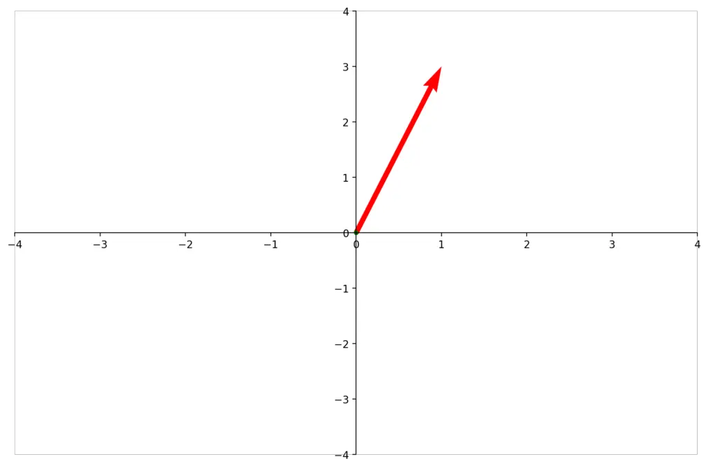
Let’s say you have a vector

\\
b =   \begin{bmatrix}
    1 \\
    3 \\
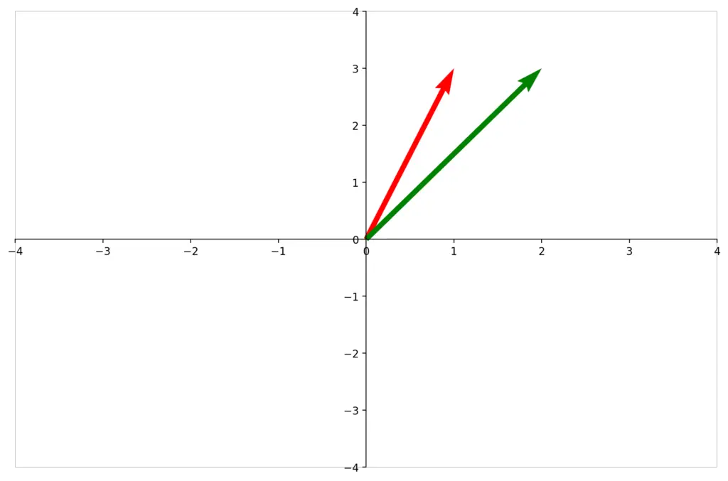
  \end{bmatrix}

Let’s say you wanted to stretch it along the x-axis by a factor of 2. You apply the transformation matrix A by taking its dot product with your vector b, resulting in the transformed vector b’.

A =   \begin{bmatrix}
    2 & 0 \\
    0 & 1 \\
  \end{bmatrix}
\\
b^’ =
\begin{bmatrix}
    2 & 0 \\
    0 & 1 \\
  \end{bmatrix}
\color{red}
  \begin{bmatrix}
    1 \\
    3 \\
  \end{bmatrix}
\color{black}
=
\color{ForestGreen}
  \begin{bmatrix}
    2 \\
    3 \\
  \end{bmatrix}

To understand why this works, you could think of the transformation matrix as transforming the basis vectors of your vector space.

In this case the x, and y axes correspond to our basis vectors.

Originally, the x and y axes are

 x = 
 \begin{bmatrix}
    1  \\
    0 \\
  \end{bmatrix}
\, y=
 \begin{bmatrix}
    0  \\
    1 \\
  \end{bmatrix}

so the transformed basis vectors can be obtained by multiplying the original vectors with the transformation matrix A.

x =

 \begin{bmatrix}
    2 & 0 \\
    0 & 1 \\
  \end{bmatrix}


   \begin{bmatrix}
   1 \\
   0 \\
  \end{bmatrix}
=

   \begin{bmatrix}
   2 \\
   0 \\
  \end{bmatrix}
\, and \,

y =

 \begin{bmatrix}
    2 & 0 \\
    0 & 1 \\
  \end{bmatrix}


   \begin{bmatrix}
   0 \\
   1 \\
  \end{bmatrix}
=

   \begin{bmatrix}
   0 \\
   1 \\
  \end{bmatrix}

Ultimately, you obtain your vector b’ in the new basis defined by A, as a linear combination of your transformed basis vectors.

\color{green}
b^{'} =
\color{red}
1
\color{black}
  \begin{bmatrix}
    2 \\
    0 \\
  \end{bmatrix}

+ 
\color{red}
3
\color{black}
  \begin{bmatrix}
    0 \\
    1 \\
  \end{bmatrix}

=
\color{green}
  \begin{bmatrix}
    2 \\
    3 \\
  \end{bmatrix}

The result is equivalent to the multiplication of the original vector b with the transformation matrix A.

\color{ForestGreen}
b^’ 
\color{black}
=
\begin{bmatrix}
    2 & 0 \\
    0 & 1 \\
  \end{bmatrix}
\color{red}
  \begin{bmatrix}
    1 \\
    3 \\
  \end{bmatrix}
\color{black}
=
\color{ForestGreen}
  \begin{bmatrix}
    2 \\
    3 \\
  \end{bmatrix}

Stretching Along the y Axis

Let’s do another example where we stretch it along the y-axis. You apply the transformation matrix.

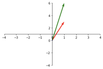
A =   \begin{bmatrix}
    1 & 0 \\
    0 & 2 \\
  \end{bmatrix}

\color{ForestGreen}
 b^{'} 
\color{black}

=
 \begin{bmatrix}
    1 & 0 \\
    0 & 2 \\
  \end{bmatrix}

\color{red}

  \begin{bmatrix}
    1 \\
    3 \\
  \end{bmatrix}

\color{black}

=
\color{ForestGreen}


  \begin{bmatrix}
    1 \\
    6 \\
  \end{bmatrix}

Of course, you could also scale along both axis at the same time.

Matrix Rotation

For now, we’ve stretched a vector along the x and y- axes. But you can do much more.

As you may have realized, in the previous section we only used diagonal transformation matrices with positive numbers. This ensured that we would only extend our vector along the x and y axes.

For example, we can mirror the vector b across the y-axis simply by turning the first entry of our transformation matrix negative.

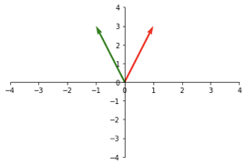
A =   \begin{bmatrix}
    -1 & 0 \\
    0 & 1 \\
  \end{bmatrix}

\color{ForestGreen}
 b^{'} 
\color{black}

=
 \begin{bmatrix}
    -1 & 0 \\
    0 & 1 \\
  \end{bmatrix}

\color{red}

  \begin{bmatrix}
    1 \\
    3 \\
  \end{bmatrix}

\color{black}

=
\color{ForestGreen}


  \begin{bmatrix}
    -1 \\
    3 \\
  \end{bmatrix}

 A 90 degree counterclockwise rotation would look like this.

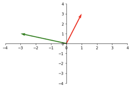
A =   \begin{bmatrix}
    0 & -1 \\
    1 & 0 \\
  \end{bmatrix}

\color{ForestGreen}
 b^{'} 
\color{black}

=
 \begin{bmatrix}
    0 & -1 \\
    1 & 0 \\
  \end{bmatrix}

\color{red}

  \begin{bmatrix}
    1 \\
    3 \\
  \end{bmatrix}

\color{black}

=
\color{ForestGreen}


  \begin{bmatrix}
    -3 \\
   1 \\
  \end{bmatrix}

Now we’ve also left the diagonal on our transformation matrix. This allows us to essentially rotate our basis vector ( and our vector space ) by 90 degrees. 

This post is part of a series on linear algebra for machine learning. To read other posts in this series, go to the index.