Probability Mass Function and Probability Density Function

In this post, we learn how to use the probability mass function to model discrete random variables and the probability density function to model continuous random variables.

Probability Mass Function: Example of a Discrete Random Variable

A probability mass function (PMF) is a function that models the potential outcomes of a discrete random variable.

For a discrete random variable X, we can theoretically list the range R of all potential outcomes since each outcome must be discrete and therefore countable.

R_x = \{x_1,x_2,x_3,...,x_k\}

Note: In statistics and probability the upper case letter X is often used to denote the conceptual random variable. The lower case letter x acts as a variable for the realized value. We speak of the probability of the conceptual variable X taking on a specific value x, where x can be any number from x1 to xk.

The probability mass function tells us how likely each specific discrete outcome is. We say that X follows the function P(X).

X  \sim  P(X)

Let’s say X can assume four distinct values x1, x2, x3, x4 that are all equally likely. The probability of X assuming the value x1 can be described in the following probability mass function of X.

P(x_1) = P(X = x_1) = \frac{1}{4}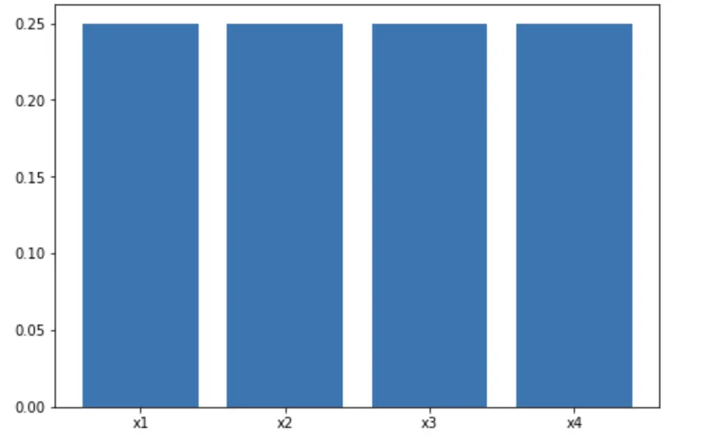

Since the probability mass function is the set of all possible values of X, the sum of all values must equal 1. One of the events is guaranteed to happen.

\sum P(x) = 1

A probability mass function can also be constructed over more than one variable. In the case of two random variables x, y, we would use the following notation.

P(X=x,Y=y)

Probability Density Function: Example of a Continuous Random Variable

A probability density function (PDF) is used to describe the outcome of a continuous random variable.

Many problems cannot be modeled with discrete random variables. If you flip a coin or throw a dice, the result will be an exact outcome. But assume you’d pick a random person in the world. What is the chance that that person is exactly 6 feet tall and not one nanometer shorter or taller? It is infinitesimally small. So rather than describing the probability of a specific discrete value, we resort to describing a region in which the probability is likely to fall.

We can construct a probability density function that gives us the probability that our outcome lies within such a region. The random variables are continuous rather than discrete.

Accordingly, we have to integrate over the probability density function. Just as with the probability mass function, the total probability is one. So the total integral over the probability function f(x) resolves to one.

\int f(x)dx = 1

The probability also needs to be non-negative.

\forall x \in X, p(x) \geq 0

Let’s say the probability that our old car survives the next couple of years follows an exponential function f(x). With every passing year, the chance that it will make it to next year shrinks exponentially.

f(x) = e^{-x}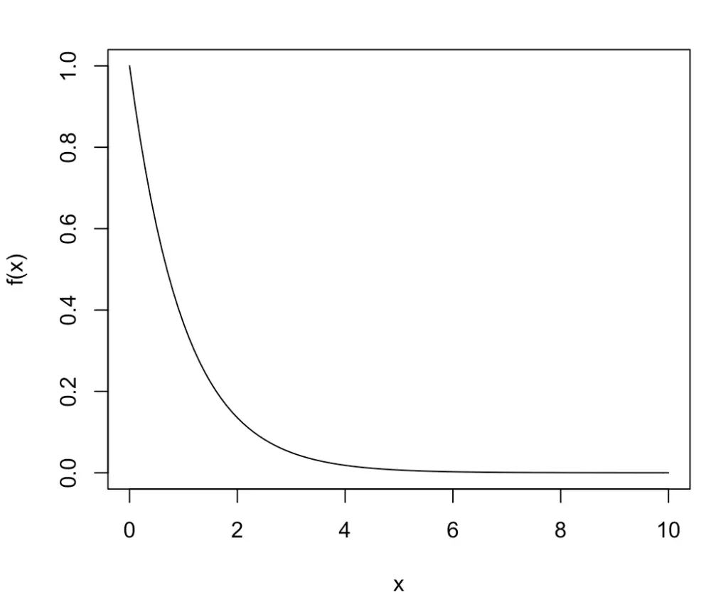

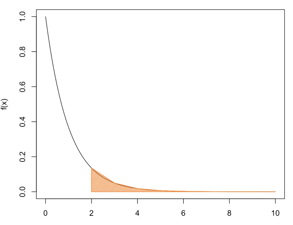
We are probably not interested in the exact time when the car breaks down for good. But we might want to know the probability that it survives for at least 2 years because by that time we will have saved enough to buy a new one.

To obtain this probability, we integrate f(x) over the interval from 2 to infinity.

\int_{2}^{\infty} f(x)dx 

This integral is fairly easy to evaluate because e doesn’t change when integrated or differentiated.

\int e^{-x}dx = e^{-x}

Now we just plug 2 and infinity into our expression and subtract them

\int_{2}^{\infty} f(x)dx = e^{-2} - e^{-\infty} = 0.135 - 0 = 0.135

Our car has a chance of roughly 13.5% of surviving at least the next two years.

A function like this one, which calculates the probability that something will last beyond a point, is also known as the survival function. We calculate the probability that our car “survives” the next two years. This is especially useful in areas like medicine where we want to know the probability of survival over a certain timeframe given a diagnosis. The survival function is defined as follows.

P(x) = P(X \gt x)

The complement of the survival function in our example is the probability that the car breaks down within the next two years.

P(x) = P(X \leq x)

This function is also known as the cumulative distribution function (CDF).

This post is part of a series on statistics for machine learning and data science. To read other posts in this series, go to the index.