The Hessian Matrix: Finding Minima and Maxima

In this post, we learn how to construct the Hessian matrix of a function and find out how the Hessian helps us determine minima and maxima.

What is a Hessian Matrix?

The Jacobian matrix helps us find the local gradient of a non-linear function. In many applications, we are interested in optimizing a function. If our function were modeling a production system, we would like to get the largest possible output for the smallest possible combination of inputs (the function variables).

The Jacobian only points us in the direction of the next local maximum, but it doesn’t tell us whether we’ve actually reached the global optimum. This problem is commonly described via the hill walking analogy:

Suppose you are walking around in the hills at night and you would like to find the highest peak. You can’t see further than a few meters because it is dark. If you followed the direction of the highest slope, you’d eventually end up on a saddle or on a hill, but it might not be the highest point. The Hessian gives you a way to determine whether the point you are standing on is, in fact, the highest hill.

How to Find the Hessian Matrix?

The Hessian matrix is a matrix of the second-order partial derivatives of a function.

df(x,y) =  
\begin{bmatrix}
    \frac{\partial^2{f(x,y)}}{\partial{x^2}} & 
     \frac{\partial^2{f(x,y)}}{\partial{xy}} 
\\
    \frac{\partial^2{f(x,y)}}{\partial{xy}} & 
     \frac{\partial^2{f(x,y)}}{\partial{y^2}} 
  \end{bmatrix}

The easiest way to get to a Hessian is to first calculate the Jacobian and take the derivative of each entry of the Jacobian with respect to each variable. This implies that if you take a function of n variables, the Jacobian will be a row vector of n entries. The Hessian will be an n \times n matrix.

If you have a vector-valued function with n variables and m vector entries, the Jacobian will be m \times n , while the Hessian will be m \times n \times n .

Let’s do an example to clarify this starting with the following function.

f(x, y) = 3x^2 + y^2

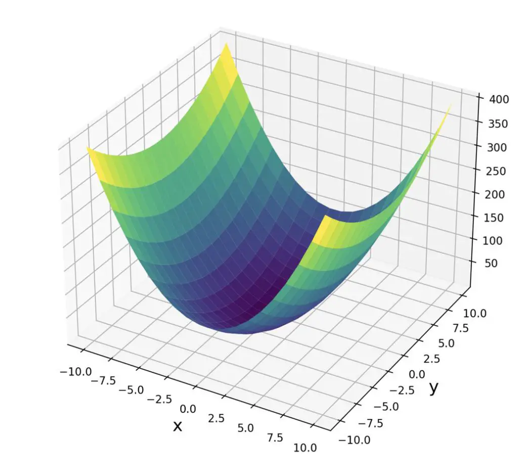
We first calculate the Jacobian.

J = \begin{bmatrix}
   6x &  2y
  \end{bmatrix}

Now we calculate the terms of the Hessian.

 \frac{\partial 6x }{\partial{x}} = 6 \; and\;
 \frac{\partial 2y }{\partial{x}} = 0  \; and\; 
 \frac{\partial 6x }{\partial{y}} = 0 \; and\; 
 \frac{\partial 2y }{\partial{y}} = 2

H = \begin{bmatrix}
   6 &  0 \\
  0 & 2
  \end{bmatrix}

Our Hessian is a diagonal matrix of constants. That makes sense since we had to differentiate twice and therefore good rid of all the exponents. We can easily calculate the determinant of the Hessian.

det(H) = 6 \times 2 - 0 \times 0 = 12

What can we infer from this information?

• If the first term in the upper left corner of our Hessian matrix is a positive number, we are dealing with a minimum.
• If the first term in the upper left corner of our Hessian matrix is negative, we are dealing with a maximum.
• In both cases, the determinant has to be positive
• If the determinant is negative, the matrix is non-definite. In this case, we might have arrived at a saddle point. We will further discuss this problem when we talk about Taylor series.

This post is part of a series on Calculus for Machine Learning. To read the other posts, go to the index.