Gamma Distribution

In this post we build an intuitive understanding of the Gamma distribution by going through some practical examples. Then we dive into the mathematical background and introduce the formulas.

The gamma distribution models the wait time until a certain number of continuously occurring, independent events have happened.

If you are familiar with the Poisson distribution and the exponential distribution, you’# realize that the Gamma distribution is very similar to the exponential distribution: In a Poisson process, the exponential distribution predicts the wait time until the first event, while the Gamma distribution predicts the wait time until the kth event.

Gamma Distribution Example

To gain an intuitive understanding of the Gamma distribution, let’s look at an example before diving into the math.

Assume you are waiting at a bus station. Busses are passing by at a rate of two per hour. You want to know the probability that you have to wait less than two hours until at least three busses have passed. The distribution of wait times for busses looks like this.

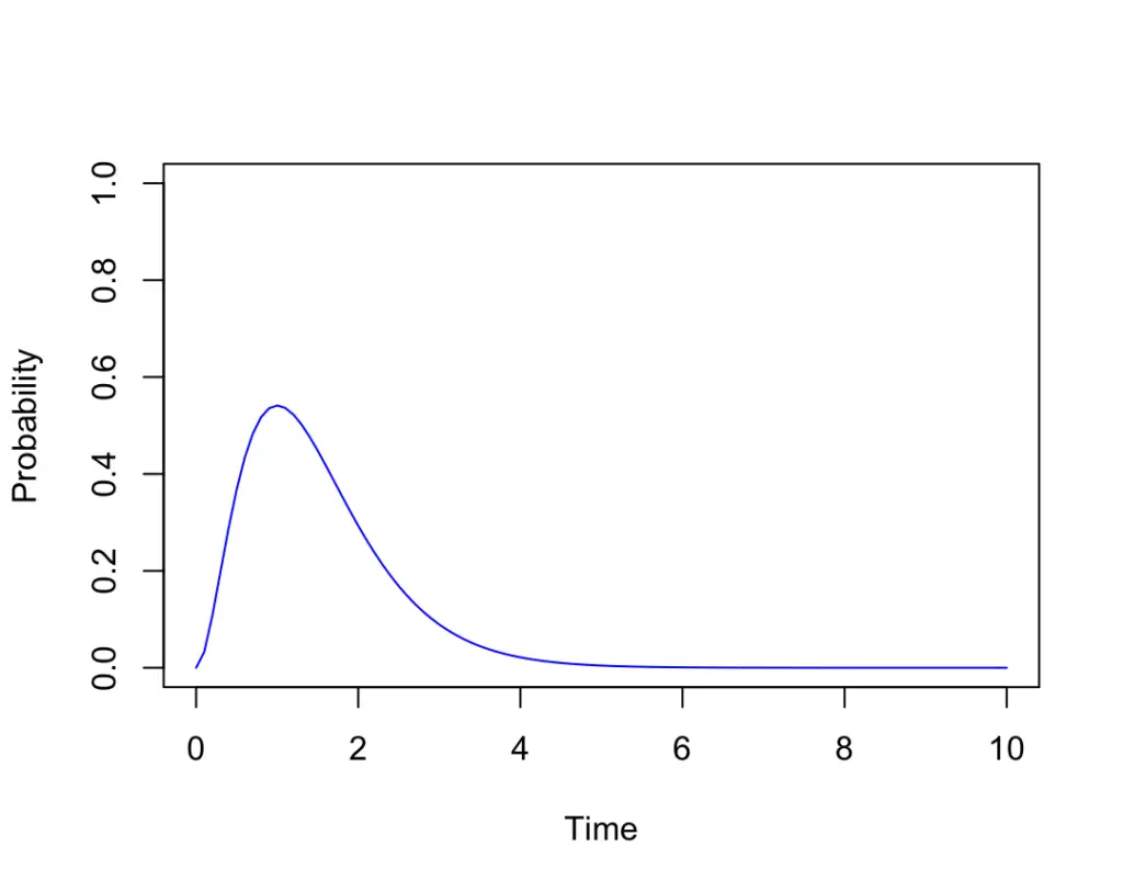
This is the probability density function of the gamma distribution. We can see that the probability for three busses passing by peaks around the 1-hour mark. But the probability of three busses passing by at one specific point in time is basically zero. It only makes sense to determine whether the busses have passed by within a certain interval. That’s why we have a probability density function.

For answering our question, the pdf is not very useful, because it is not cumulative.

We want to know how likely it is that three busses pass by within 2 hours, So we need to add up all the probabilities that three busses pass for every point in time between zero and 2 hours. That’s what we have a cumulative distribution function for.

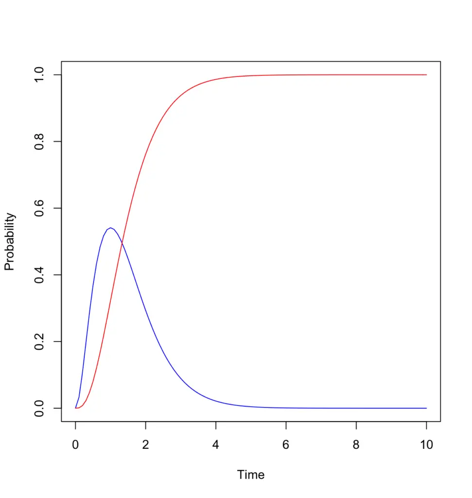
Judging from the shape of the cumulative distribution function, the probability that 3 busses have passed at the 2-hour mark given an average rate of 2 busses per hour, looks like it is around 70% – 80%.

Let’s calculate the actual probability using the formula for the gamma distribution.

Gamma Distribution Formula

A gamma distribution is parameterized by two variables α, and β.

α is known as the shape parameter. In our example it is 3, the number of busses we wish to observe.

β is the rate parameter and it is equivalent to lambda in the Poisson distribution. In our example, it is 2, the rate of basses passing per time unit (hours in our example).

The variable x denotes the desired wait time (2 hours in our example). Γ is the greek letter Gamma. In the gamma distribution, it denotes the factorial of alpha – 1,

Some definitions also parameterize the gamma distribution using k and theta. The difference is that instead of using beta, it uses theta, which is the inverse of beta. For simplicity’s sake, we’ll stick with the alpha, beta parameterization.

PDF of the Gamma Distribution

Here is the formula for the probability density function.

f(x; \alpha, \beta) = \frac{\beta^{\alpha} x^{\alpha - 1} e^{-\beta x}}{\Gamma(\alpha)}

\Gamma(\alpha) = (\alpha -1)!

CDF of the Gamma Distribution

The cumulative distribution function is obtained by integrating the probability density function with respect to x. I won’t go through the steps of the integration but give you the formula straight away. Provided that α is a positive integer, the CDF looks like this.

F(x; \alpha, \beta) = 1 - \sum_{i=0}^{\alpha-1} \frac{(\beta x)^i e^{-\beta x}}{i!}

If we plug our values into the formula, we get a value of roughly 76%.

F(x; \alpha, \beta) = 0.76

The probability that 3 busses have passed by after two hours is 76% when the average arrival rate is 2 busses per hour.

Some more Examples

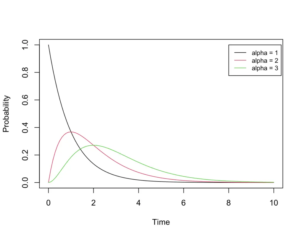
The Gamma distribution is a bit hard to grasp at first, so let’s look at how the distribution changes when we vary parameters. Let’s start by varying the parameter lambda.

I find the CDF easier to interpret than the PDF. Here it is.

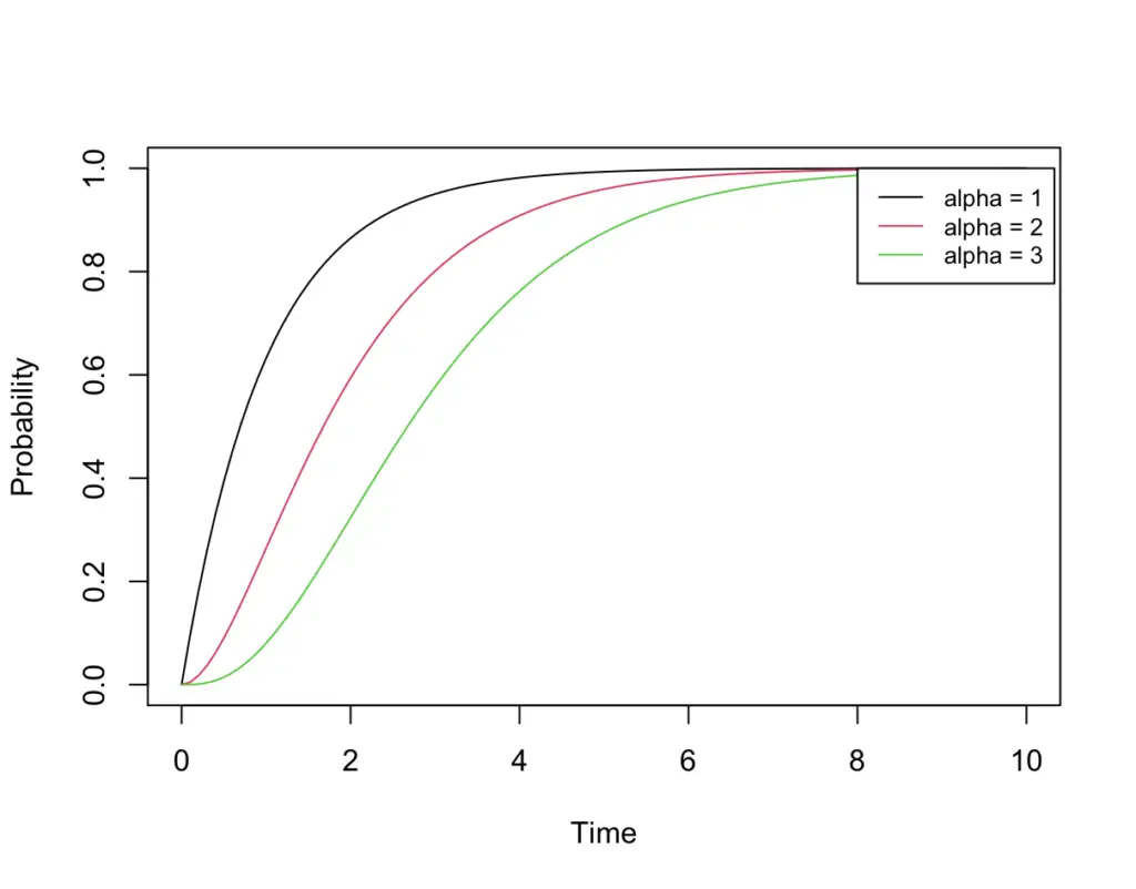
As alpha increases, the CDF is less steep. This makes sense. If we are waiting for 1 bus to pass with busses arriving at a rate of one per hour, the probability that we have observed at least one bus after 2 hours is very high.

If we are waiting for for3 busses to pass by while the rate at which busses arrive stays the same at one per hour, the probability that at least 3 busses have passed at the 2-hour mark is much lower.

On the other hand, if we increase beta, that is, increase the rate at which busses pass while keeping alpha constant, we get this for our PDF.

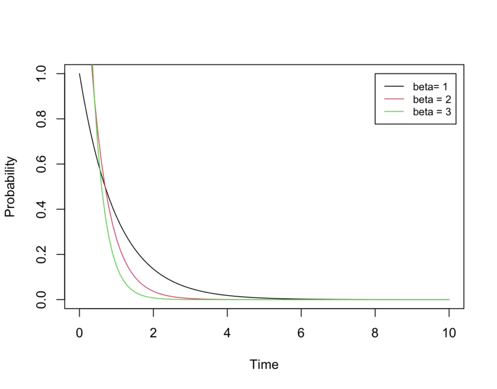
And this is our CDF.

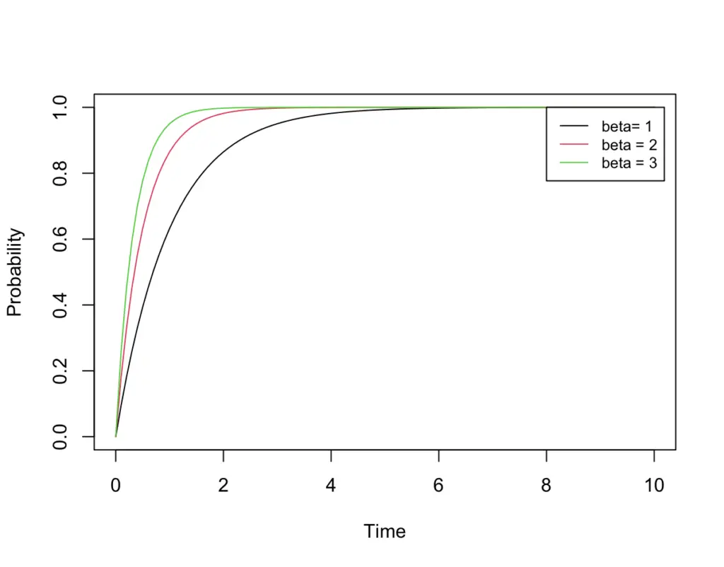
If busses pass at a rate of 3 per hour, the probability of observing at least one bus peaks earlier than if they were passing at a rate of one per hour.

This post is part of a series on statistics for machine learning and data science. To read other posts in this series, go to the index.