Principal Components Analysis Explained for Dummies

In this post, we will have an in-depth look at principal components analysis or PCA. We start with a simple explanation to build an intuitive understanding of PCA. In the second part, we will look at a more mathematical definition of Principal components analysis.
Lastly, we learn how to perform PCA in Python.

What is Principal Components Analysis (PCA)

Principal Components Analysis, also known as PCA, is a technique commonly used for reducing the dimensionality of data while preserving as much as possible of the information contained in the original data. PCA achieves this goal by projecting data onto a lower-dimensional subspace that retains most of the variance among the data points.

What is dimensionality reduction, and what is a subspace? Let’s illustrate this with an example.

If you have data in a 2-dimensional space, you could project all the data points onto a line using PCA.

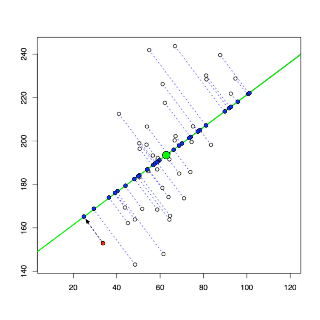
You have essentially reduced the dimensionality of your data from 2D to 1D.
The 1D space (your line) is a subspace of the 2D coordinate system.

The green line has been constructed using mathematical optimization to maximize the variance between the data points as much as possible along that line.
We call this line our first principal component. Naturally, the points on the line are still closer to each other than in the original 2D space because you are losing a dimension to distinguish them. But in many cases, the simplification achieved by dimensionality reduction outweighs the loss in information, and the loss can be partly or fully reconstructed.

Imagine you are taking a photo of some people. You are reducing the dimensionality from 3D (the real world) to a 2D representation. You are losing some explicit 3D information, such as the distance between a person in the front and another person further in the back. However, you will have a pretty decent idea of how far these two persons are apart in reality because the person in the back will appear smaller than the person in the front. So the 3D information is not completely lost but sort of encoded in the 2D image.

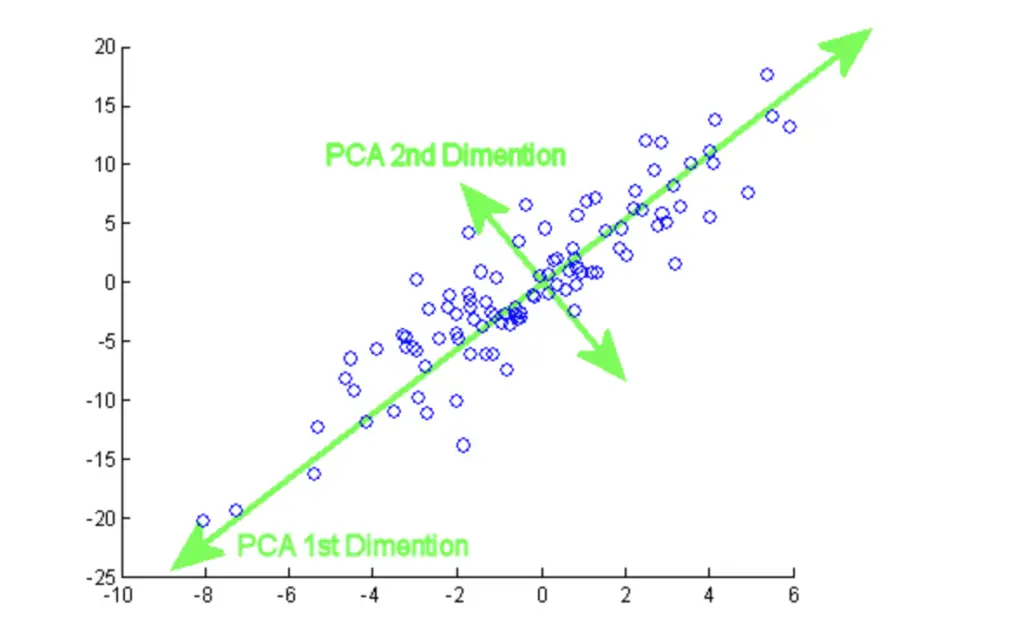
In our previous example, we only had one principal component. Once you move into higher dimensional spaces, you’ll likely use several principal components because the variance explained by one principal component is often insufficient. Principal components are vectors that are orthogonal to each other. This means they form a 90-degree angle. Mathematically, orthogonal vectors are independent, meaning the variance explained by the second principal component does not overlap with the variance of the first. So they represent information as efficiently as possible.
The first principal component will capture most of the variance; the second principal component will capture the second-largest part of the variance that has been left unexplained by the first one, etc.

Practically speaking, principal components are feature combinations that represent the data and its differences as efficiently as possible by ensuring that there is no information overlap between features. The original features often display significant redundancy, which is the main reason why principal components analysis works so well at reducing dimensionality.

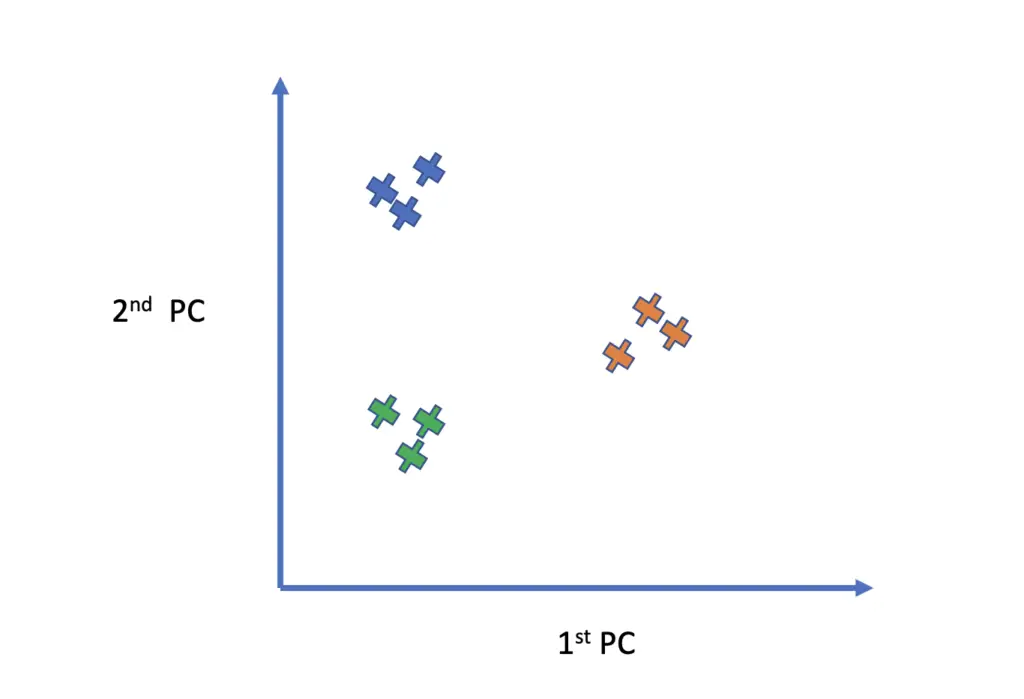
If you plot your data in your lower-dimensional subspace with the principal components as your axes, similar data points should cluster together. This happens because you are explicitly focusing on axes that maximize the variance.

In highly dimensional datasets, the vast majority of the variance in the data is often captured by a small number of principal components. A plot of the distribution of the variance across principal components may look like this.

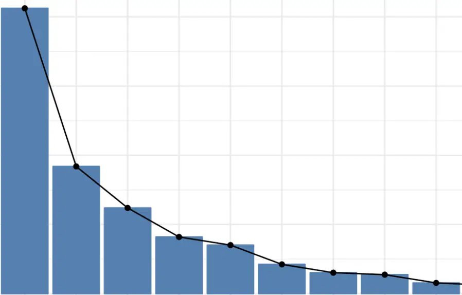
As you can see, the first principal component explains vastly more than the following ones. This allows us to project even highly dimensional data down to relatively low-dimensional subspaces.

How does Principal Components Analysis Work?

Principal Components Analysis achieves dimensionality reduction through the following steps.

1. Standardize the data

The variables that make up your dataset will often have different units and different means. This can cause issues such as producing extremely large numbers during the calculation. To make the process more efficient, it is good practice to center the data at mean zero and make it unit-free. You achieve this by subtracting the current mean from the data and dividing by the standard deviation. This preserves the correlations but ensures that the total variance equals 1.

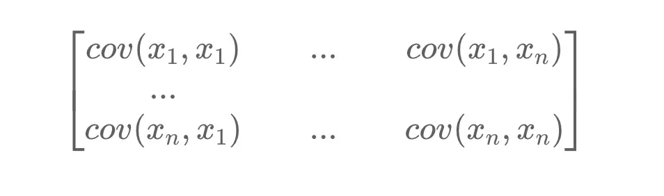
2. Calculate the Covariance Matrix

Principal components analysis attempts to capture most of the information in a dataset by identifying the principal components that maximize the variance between observations. The covariance matrix is a symmetric matrix with rows and columns equal to the number of dimensions in the data. It tells us how the features or variables diverge from each other by calculating the covariance between the pairwise means.

If you want to learn more about covariance matrices, I suggest you check out my post on them.

3. Calculate the Eigenvectors and Eigenvalues of the Covariance Matrix

Eigenvectors are linearly independent vectors that do not change direction when a matrix transformation is applied. Eigenvalues are scalars that indicate the magnitude of the Eigenvector. If you want to learn more, check out my post on Eigenvectors and Eigenvalues.

The Eigenvectors of the covariance matrix point in the direction of the largest variance. The larger the Eigenvalue, the more of the variance is explained. In other words, the Eigenvector with the largest Eigenvalue corresponds to the first principal component, which explains most of the variance, the Eigenvector with the second-largest Eigenvalue corresponds to the second principal component, etc.

The reason why Eigenvectors correspond to principal components is buried in an elaborate mathematical proof which we will tackle in the next section. But in this section, we focus on intuition rather than complicated proofs, so for now, we just take this relationship for granted.

4. Reduce Dimensionality

As stated previously, the principal components are efficient feature combinations that ensure that the information explained does not overlap between features. Eliminating information redundancy already helps in reducing dimensionality. But since the percentage of the overall variance explained declines with every new principal component, we can reduce dimensionality further by eliminating the least important principal components. At this stage, we have to decide how many principal components are sufficient and how much information loss we can tolerate.

Lastly, we need to project the data from our original feature space down to the reduced space spanned by our principal components.

Usually, you will perform principal components analysis using a software tool that will execute all the steps for you. In this case, a high-level understanding as presented up until here is usually enough. But if you are interested in the mathematical details that explain why PCA works and why Eigenvectors represent principal components, read on.

Why does Principal Components Analysis Work?

This section dives into the mathematical details of principal components analysis. To be able to follow along, you should be familiar with the following mathematical topics. I’ve linked each topic to a corresponding post on this blog with an explanation of the topic. All links open in a new tab so you’ll stay on this post.

• Matrix Transformations
• Eigenvectors and Eigenvalues
• Partial derivatives
• Lagrange multipliers
• Variance and Covariance

Given a D-dimensional dataset with features X = {x_1, x_2, …, x_N} we want to find a K-dimensional representation of the dataset where K < D.

This requires us to find a K-dimensional subspace of D and a corresponding projection matrix B. so that multiplication of our existing features X = {x_1, x_2, …, x_N} with B will result in the K-dimensional representation of our dataset.

For the sake of simplicity, let’s say we want to project onto a 1-dimensional subspace (K=1). Accordingly, our projection matrix becomes 1-dimensional which implies that our matrix B turns into a vector b_1.

Our problem now is fairly straightforward. We want to find a 1-dimensional representation Z = {z_1, z_2, …, z_N} of the data points X = {x_1, x_2, …, x_N} which is achieved by multiplying with the projection vector b. To be able to multiply the two, we need the transpose of b.

z_{1n} = b_1^Tx_n

Z basically represents the coordinate in X projected onto a 1-dimensional subspace.

The principal components obtained through the eigenvectors lead us to the representation Z that maximizes the variance of the observations in X.
Mathematically, our goal is thus to find the maximum variance representation of the coordinates in Z. Just like with X; we obtain the variances by calculating the sum of the squares of the observations in Z and dividing by the number of observations in Z.

V_1 = \frac{1}{N} \sum_{n=1}^N z^2_{1n}

Since we don’t know the observations in Z yet, we replace them with the previous expression of z through b and x.

V_1 = \frac{1}{N} \sum_{n=1}^N (b_1^Tx_n)^2 

Exploiting the symmetry of the expression

b_1^T x_n =  x_n^T b_1

V_1 = \frac{1}{N} \sum_{n=1}^N (b_1^Tx_n x_n^T b_1) = b_1^T \left(\frac{1}{N} \sum_{n=1}^N (x_n x_n^T )\right) b_1

To simplify things a bit, we replace the inner term with the matrix C. C also represents the covariance matrix of the observations in X.

C = \frac{1}{N}\sum_{i=1}^{N} x_nx_n^T

So we get

V_1 = b_1^T C b_1

Since the goal is to find the vector b that maximizes the variance, we can turn this into an optimization problem that we solve by partially differentiating with respect to b and setting the expression equal to zero. But we still need one more constraint in place. The norm of b needs to be restricted to unit length. Otherwise, the variance might explode to infinity.

x_1x_1^T =  ||x_1||^2 = 1

Using a LaGrange multiplier lambda, we can now set up our optimization problem where we like to find optimum values for b and lambda.

 f(b_1, \lambda) =  b_1^T C b_1 + \lambda_1( b_1^T b_1 - 1)

The vector b corresponds to our Eigenvector, while lambda corresponds to the Eigenvalue. Remember that the Eigenvector associated with the largest Eigenvalue equals the principal component that explains most of the variance.

To solve the equations, we differentiate with respect to lambda, which gives us the following expression for the Eigenvalue.

\frac{\partial f}{\partial \lambda_1} = b_1^T b_1 - 1 = 0

b_1^T b_1 = 1

And we arrive at the following expression for the Eigenvector b by differentiating with respect to b.

\frac{\partial f}{\partial b_1} = 2b_1C - 2\lambda_1 b_1^T = 0

b_1C = \lambda_1 b_1^T

We can plug these results into our original expression for the variance.

V_1 = b_1^T C b_1 = \lambda_1 b_1^T b_1 = \lambda_1

In other words, the variance is equivalent to the Eigenvalue associated with the Eigenvector that spans the 1-dimensional subspace and therefore corresponds to the principal component.

Once we get to higher dimensional subspaces, the same idea applies. When projecting onto a K-dimensional subspace, we can construct K principal components. The kth Eigenvalue λ_k associated with the kth Eigenvector b_k corresponds to the kth part of the variance (remember that PCA splits the total variance into non-overlapping parts).

V_k = b_k^T C b_k = \lambda_k b_k^T b_k = \lambda_k

The amount of the total variance captured by k principal components becomes a simple sum over k Eigenvalues.

V_K = \sum_{k=1}^K = \lambda_K

Principal Components Analysis in Python

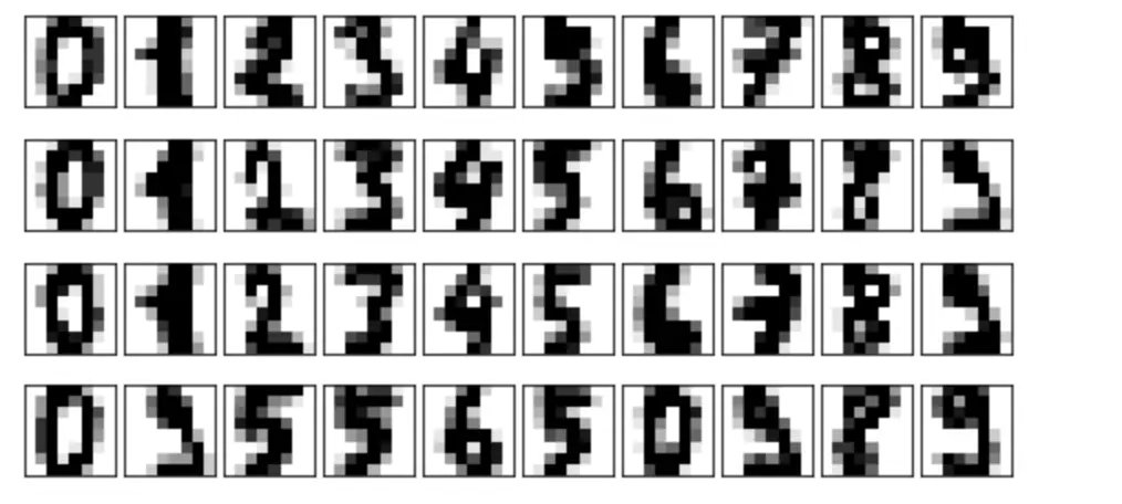
In this section, we use PCA to reduce the dimensionality of the digits dataset. The digits dataset consists of 1797 8×8 images of handwritten digits. Each 8×8 image is transformed into a feature matrix of 64 features.
I’ve adapted the code from an example in the “Python Data Science Handbook”.

We start by importing the relevant packages.

import numpy as np
import matplotlib.pyplot as plt
from sklearn.datasets import load_digits
from sklearn.decomposition import PCA
%matplotlib inline

Next, we load the digits and look at their dimensions. As expected, we have a dataset that consists of 1797 images, each of which has 64 features.

digits = load_digits()
digits.data.shape. # (1797, 64)

With the following function, we can visualize the digits.

def plot_digits(data):
    fig, axes = plt.subplots(4, 10, figsize=(8, 4),
                             subplot_kw={'xticks':[], 'yticks':[]},
                             gridspec_kw=dict(hspace=0.1, wspace=0.1))
    for i, ax in enumerate(axes.flat):
        ax.imshow(data[i].reshape(8, 8),
                  cmap='binary', interpolation='nearest',
                  clim=(0, 10))

#run the function
plot_digits(digits.data)

Let’s use principal components analysis to project the data from a 64-dimensional space down to a 2-dimensional space so that we can visualize the distribution on a 2-D plot.

We already imported the PCA algorithm from the SciKitLearn package. Now we have to initialize it and specify the number of principal components we’d like to retain. Next, we fit the PCA algorithm to the data and transform it to a 2-D space using the fit_transform function.

pca = PCA(n_components=2)  # project from 64 to 2 dimensions
reduced = pca.fit_transform(digits.data)

print(reduced.shape) #(1797, 2)

What is the difference between Fit and Fit_Transform?

If you play with Python’s PCA package, you will come across a fit, a transform, and a fit_transform function. How do they differ?

The “Fit” function only fits the data and returns a PCA model that can be applied to new data. The transform “method” can only be called on a fit model, and it returns the transformed data. Thransform_fit performs fitting and data transform at once.

This piece of code gives us the same result as the previous one.

pca = PCA(n_components=2)  # project from 64 to 2 dimensions
fit_pca = pca.fit(digits.data)
reduced = fit_pca.transform(digits.data)
print(reduced.shape) (1797, 2)

Calling only fit is appropriate if you want your PCA algorithm to learn how to do transforms on one dataset but want to apply the trained algorithm to another dataset by calling transform.

Visualizing the Data

We have reduced the dimensionality of our data from 64 to two, so we can visualize it on a 2D grid.

plt.scatter(reduced[:, 0], reduced[:, 1],
            c=digits.target, edgecolor='none', alpha=0.5,
            cmap=plt.cm.get_cmap('Accent', 10))
plt.xlabel('PC 1')
plt.ylabel('PC 2')
plt.colorbar();

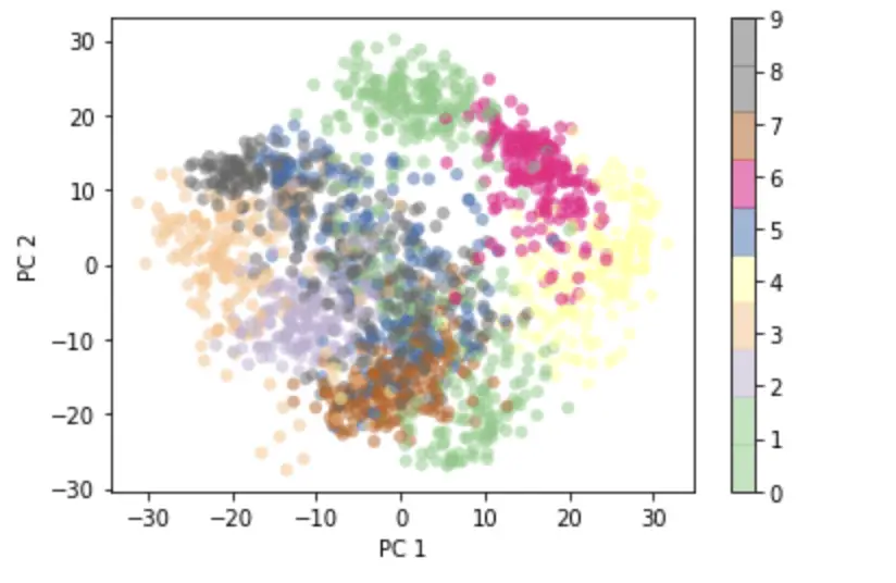
This is the 2-D representation of the 64-dimensional images that captures the largest amount of possible information. Digits that look similar cluster together on the 2D grid.

How much of the variance is actually retained by the individual principal components. We can find this out using Python.

print(pca.explained_variance_ratio_) #[0.14890594 0.13618771]

It seems like the first two principal components capture almost 30% of the variance contained in the original 64-dimensional representation.

As an experiment, let’s fit PCA again without reducing the number of components and see how much of the variance each component explains. Tho do that, we initialize PCA without specifying the number of components and fit it to the digits data. Then we visualize the distribution of the explained variance across all 64 components.

pca = PCA().fit(digits.data)
plt.plot(pca.explained_variance_ratio_)
plt.xlabel('number of components')
plt.ylabel('explained variance');

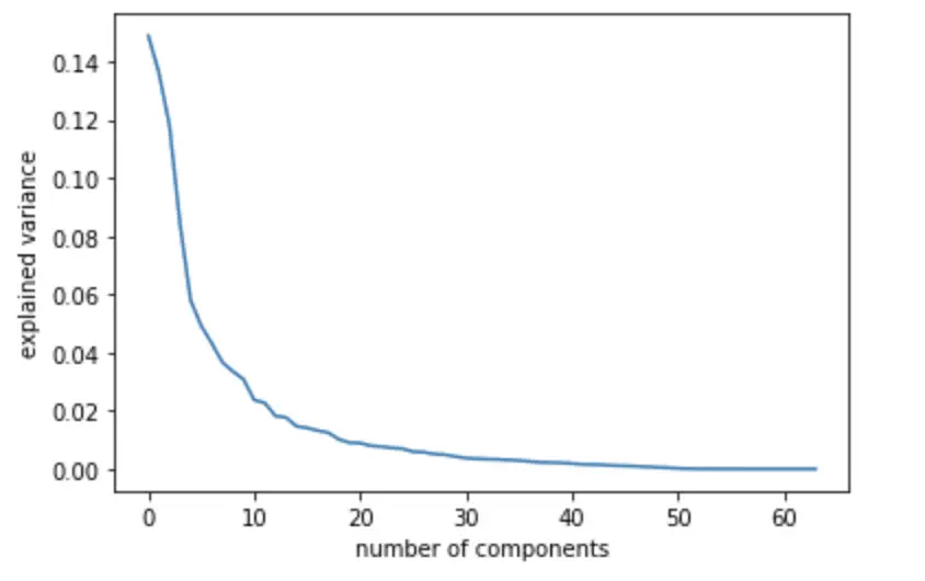
The variance explained declines sharply with each additional principal component. It appears that almost all of the variance is captured by the first 10 components. This is very useful in practice as it allows us to reduce the dimensionality down to one-sixth of the original data without losing a significant amount of information.

If you want a more in-depth explanation with hands-on practice labs in Python, I suggest checking out this Imperial College PCA course on Coursera.

This post is part of a larger series I’ve written on machine learning and deep learning. For a comprehensive introduction to deep learning, check out my blog post series on neural networks. My series on statistical machine learning techniques covers techniques such as linear regression, logistic regression, and support vector machines.