Understanding Eigenvectors in 10 Minutes

In this post, we explain the concept of eigenvectors and eigenvalues by going through an example.

What are Eigenvectors and Eigenvalues

An eigenvector of a matrix A is a vector v that may change its length but not its direction when a matrix transformation is applied. In other words, applying a matrix transformation to v is equivalent to applying a simple scalar multiplication. A scalar can only extend or shorten a vector, but it cannot change its direction.

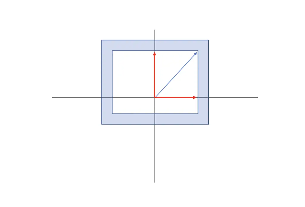
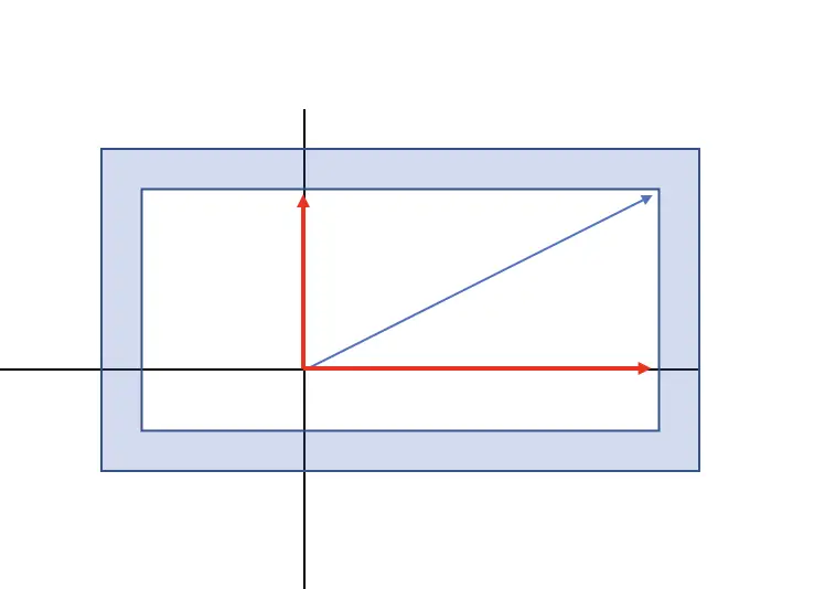
If you scale the plane on the left along the x-axis, the two red vectors are eigenvectors, while the blue one is not.

The red vector that runs parallel to the x-axis only extends its length but does not change its direction, while the red vector along the y axis does not change at all. The blue vector, on the other hand, also changes its direction.

The eigenvalue describes the scalar, by which the eigenvectors are multiplied to achieve the vector of the desired length.

Whether a vector is an eigenvector depends on the type of matrix transform applied. For example, if you apply a rotation other than 180 degrees, all vectors need to be multiplied with a matrix to achieve the desired change in direction. Multiplying by a scalar is not enough.

How to Find Eigenvalues

As stated previously, multiplying an Eigenvector v by the transformation matrix A can also be achieved by simply multiplying v by a scalar λ, where λ corresponds to our eigenvalue. Accordingly, we can say:

Av = \lambda v

Now we can rearrange this system into the following equation by simply bringing λv to the left.

(A - \lambda I)v = 0

If we take v out, we also have to multiply λ by the identity matrix of A to maintain the same dimensions as A.

Finding the eigenvectors now requires us to find a non-trivial solution for this equation. If v were zero, the equation would resolve to zero, but we wouldn’t be able to obtain λ. This is a trivial solution that we are not interested in. Instead, we need to find the solution for which the term in brackets resolves to zero. We discussed previously that a matrix’s determinant is zero if its column vectors do not span a plane (that is if they have the same direction). Accordingly, we can resolve the expression in the brackets by setting its determinant equal to zero.

det(A - \lambda I) =  0

 det(
 \begin{bmatrix}
    a & b \\
    c & d \\
  \end{bmatrix} 
- 
  \begin{bmatrix}
    \lambda & 0 \\
    0 & \lambda \\
  \end{bmatrix}
)
=
 det(
 \begin{bmatrix}
    a- \lambda & b \\
    c & d - \lambda\\
  \end{bmatrix} 
)
=
0

If we multiply this out, we arrive at the characteristic polynomial.

(a- \lambda)(d- \lambda) -bc = \lambda^2- (a+d)\lambda + ad - bc = 0

Now we need to plug in the terms from our matrix A (a,b,c,d), and we can obtain lambda.

How to Find Eigenvectors

Now that we have the eigenvalues finding the eigenvectors requires us to plug the eigenvalues into our original equation.

(A - \lambda I)v = 0

 \begin{bmatrix}
    a- \lambda & b \\
    c & d - \lambda\\
  \end{bmatrix} 
 \begin{bmatrix}
     v_1 \\
     v_2 \\
  \end{bmatrix} 
= 0

Let’s do an example where we scale a vector v by the following matrix A.

A =
 \begin{bmatrix}
    3 & 0 \\
    0 & 1\\
  \end{bmatrix} 

(
 \begin{bmatrix}
    3 & 0 \\
    0 & 1\\
  \end{bmatrix} 
-
\lambda

 \begin{bmatrix}
    1 & 0 \\
    0 & 1\\
  \end{bmatrix} 
)v
= 0

Now our characteristic polynomial resolves to the following.

\lambda^2 - 4\lambda + 3 = 0 

Lambda now has two real solutions, which are our eigenvalues:

\lambda = 1 \\ \lambda = 3

To obtain our eigenvectors, we plug the Eigenvalues back into our original expression.

(
 \begin{bmatrix}
    3 & 0 \\
    0 & 1\\
  \end{bmatrix} 
-
1
 \begin{bmatrix}
    1 & 0 \\
    0 & 1\\
  \end{bmatrix} 
)v
= 
 \begin{bmatrix}
    2 & 0 \\
    0 & 0\\
  \end{bmatrix} 
 \begin{bmatrix}
    v_1 \\
    v_2 \\
  \end{bmatrix} 
=

 \begin{bmatrix}
    2 v_1 \\
    0\\
  \end{bmatrix}  
=
0

(
 \begin{bmatrix}
    3 & 0 \\
    0 & 1\\
  \end{bmatrix} 
-
3
 \begin{bmatrix}
    1 & 0 \\
    0 & 1\\
  \end{bmatrix} 
)v
= 
 \begin{bmatrix}
    0 & 0 \\
    0 & -2\\
  \end{bmatrix} 
 \begin{bmatrix}
    v_1 \\
    v_2 \\
  \end{bmatrix} 
=

 \begin{bmatrix}
    0 \\
    -2v_2\\
  \end{bmatrix} 

In the first case, v1 needs to equal zero (because 2v1 = 0), but for v2 we only have the generic expression 0 = 0. This holds regardless of what value v2 assumes. Accordingly, v2 can take any value as long as v1 remains 0.

In the second case, it is exactly the other way around. The vector v1 can assume any value as long as v2 is zero.

This makes sense because A scales v along an axis but doesn’t shear or rotate it. Accordingly, the eigenvectors extend or contract along that same axis.

What happens if we wanted to do a transformation that has no real Eigenvalues and Eigenvectors? In this case, the characteristic polynomial won’t have a solution in the real number space. We could still solve it with complex eigenvalues and complex eigenvectors.

This post is part of a series on linear algebra for machine learning. To read other posts in this series, go to the index.