An Introduction to Neural Network Loss Functions

This post introduces the most common loss functions used in deep learning.

The loss function in a neural network quantifies the difference between the expected outcome and the outcome produced by the machine learning model. From the loss function, we can derive the gradients which are used to update the weights. The average over all losses constitutes the cost. To understand how the gradients are calculated and used to update the weights, refer to my post on backpropagation with gradient descent.

A machine learning model such as a neural network attempts to learn the probability distribution underlying the given data observations. In machine learning, we commonly use the statistical framework of maximum likelihood estimation as a basis for model construction. This basically means we try to find a set of parameters and a prior probability distribution such as the normal distribution to construct the model that represents the distribution over our data. If you are interested in learning more, I suggest you check out my post on maximum likelihood estimation.

Cross-Entropy based Loss Functions

Cross-entropy-based loss functions are commonly used in classification scenarios. Cross entropy is a measure of the difference between two probability distributions. In a machine learning setting using maximum likelihood estimation, we want to calculate the difference between the probability distribution produced by the data generating process (the expected outcome) and the distribution represented by our model of that process.
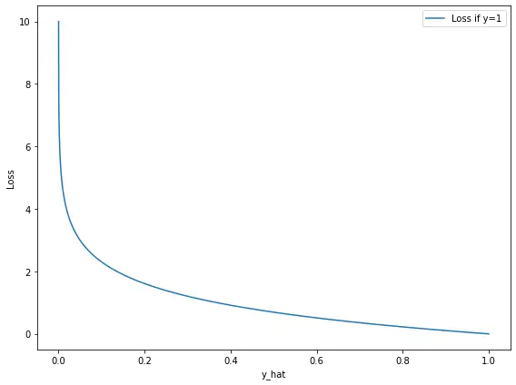
The resulting difference produced is called the loss. It increases exponentially as the prediction diverges from the actual outcome.

If the actual outcome is 1, the model should produce a probability estimate that is as close as possible to 1 to reduce the loss as much as possible.

If the actual outcome is 0, the model should produce a probability estimate that is as close as possible to 0.

As you can see on the plot, the loss explodes exponentially, preventing the model from reaching a prediction equal to 1 (absolute certainty in the wrong value). Conversely, the closer the estimate gets to the actual outcome, the more the returns diminish.

Cross entropy is also referred to as the negative log-likelihood.

Binary Cross-Entropy

As the name implies, the binary cross-entropy is appropriate in binary classification settings to get one of two potential outcomes. The loss is calculated according to the following formula, where y represents the expected outcome, and y hat represents the outcome produced by our model.

L = -(y_i \; log(\hat y_i) + (1-y_i)log(1-\hat y_i))

To make this concrete, let’s go through an example.

Let’s say you are training a neural network to determine whether a picture contains a cat. The outcome is either 1 (there is a cat) or 0 (there is no cat). You have 2 pictures, the first two of which contain cats, while the last one does not. The neural network is 80% confident that the first image contains a cat.

y = 1 \\
\hat y = 0.8

If we plug the first estimate and the expected outcome into our cross-entropy loss formula, we get the following:

L = -(1 \; log( 0.8) + (1-1)log(1-0.8)) = 0.32

The neural network is 10% confident that the second image contains a cat. In other words, the neural network gives you a 90% probability that the second image does not contain a cat.

y = 0 \\
\hat y = 0.1

If we plug the last estimate and expected outcome into the formula, we get the following.

L = -(0 \; log( 0.1) + (1-0)log(1-0.1)) = 0.15

The function is designed so that either the first or the second term equals zero. You attain the cost by calculating the average over the loss overall examples.

C = -\frac{1}{N} \sum_{i=1}^{N}(y_i \; log(\hat y_i) + (1-y_i)log(1-\hat y_i))

The binary cross-entropy is appropriate in conjunction with activation functions such as the logistic sigmoid that produce a probability relating to a binary outcome.

Categorical Cross-Entropy

The categorical cross-entropy is applied in multiclass classification scenarios. In the formula for the binary cross-entropy, we multiply the actual outcome with the logarithm of the outcome produced by the model for each of the two classes and then sum them up. For categorical cross-entropy, the same principle applies, but now we sum over more than two classes. Given that M is the number of classes, the formula is as follows.

L = \sum^M_{j=1} y_j\log(\hat y_j)

Assume that we have a neural network that learns to classify pictures into three classes: Whether they contain a rabbit, a cat, or a dog. To represent each sample, your expected outcome y is a vector of three entries for each class. The entry that corresponds to the outcome is 1, while all others are zero. Let’s say the first image contains a dog.

y = \begin{bmatrix}
1\\
0\\
0
\end{bmatrix}

The vector of predictions contains probabilities for each outcome that need to sum to 1.

\hat y = \begin{bmatrix}
0.7\\
0.2\\
0.1
\end{bmatrix}

To calculate the loss for this particular image of a dog, we plug these values into the formula.

L = 1\log(0.7) + 0\log(0.2)+0\log(0.1) = 0.52

For the cost function, we need to calculate the loss of all the individual training examples.

L = -\frac{1}{N} \sum_{i=1}^{N}\sum^M_{j=1} y_{ij}\log(\hat y_{ij})

The categorical cross-entropy is appropriate in combination with an activation function such as the softmax that can produce several probabilities for the number of classes that sum up to 1.

Sparse Categorical Cross-Entropy

In deep learning frameworks such as TensorFlow or Pytorch, you may come across the option to choose sparse categorical cross-entropy when training a neural network.

Sparse categorical cross-entropy has the same loss function as categorical cross-entropy. The only difference is how you present the expected output y. If your y’s are in the same format as above, where every entry is expressed as a vector with 1 for the outcome and zeros everywhere else, you use the categorical cross-entropy. This is known as one-hot encoding.

If your y’s are encoded in an integer format, you would use sparse categorical cross-entropy. In the example above, a dog could be represented by 1, a cat by 2, and a rabbit by 3 in integer format.

Mean Squared Error

Mean squared error is used in regression settings where your expected and your predicted outcomes are real-number values.

The formula for the loss is fairly straightforward. It is just the squared difference between the expected value and the predicted value.

L =  (y_i - \hat y_i)^2

Suppose you have a model that helps you predict the price of oil per gallon. If the actual price of the house is $2.89 and the model predicts $3.07, you can calculate the error.

L = (2.89 - 3.07)^2 = 0.032

The cost is again calculated as the average overall losses for the individual examples.

C = \frac{1}{N} \sum_{i=1}^N (y_i - \hat y_i)^2

Further Resources

This post is part of a larger series I’ve written on machine learning and deep learning. For a comprehensive introduction to deep learning, check out my blog post series on neural networks. My series on statistical machine learning techniques covers techniques such as linear and logistic regression.

As a general beginner resource for studying neural networks, I highly recommend Andrew Ng’s deep learning specialization on Coursera. It has recently been updated with new material.