Understanding the Change of Basis Matrix

In this post, we learn how to construct a transformation matrix and apply it to transform vectors into another vector space. This process is also referred to as performing a change of basis.

As discussed in the previous article on vector projections, a vector can be represented on a different basis than the basic coordinate system.

What is a Change of Basis Matrix?

A change of basis matrix is a matrix that translates vector representations from one basis, such as the standard coordinate system, to another basis. A change of basis matrix also allows us to perform transforms when the new basis vectors are not orthogonal to each other.

This sounds fairly abstract, so let’s go through an example to make it clearer.

Given our standard coordinate system consisting of the basis vectors

  \begin{bmatrix}
    1 \\
    0 \\
  \end{bmatrix}
\,
and
\,
  \begin{bmatrix}
    0 \\
    1 \\
  \end{bmatrix}

we have an alternative vector space consisting of the blue basis vectors, and a vector b represented in coordinates of that alternative vector space.

\color{blue}
basis: 
  \begin{bmatrix}
    1 \\
    2 \\
  \end{bmatrix}
\,
and
\,
  \begin{bmatrix}
    3 \\
    1 \\
  \end{bmatrix} \\

\color{red}
b =   \begin{bmatrix}
    1 \\
    1 \\
  \end{bmatrix}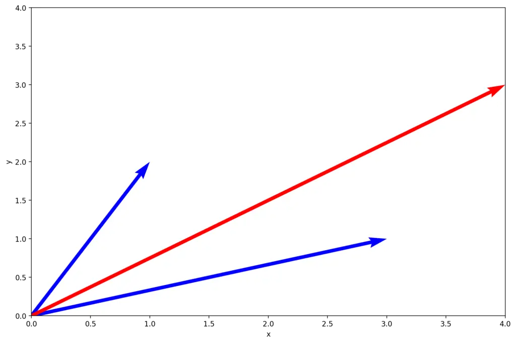

Notice, that the blue vectors are not linearly independent. Accordingly, the method we learned previously using the dot product, won’t work here. But the basis vectors of our blue basis form a matrix, which we can use transform b from the alternative basis into our standard coordinate system as follows:

\color{blue}
\begin{bmatrix}
1 &3 \\
2 & 1 \\
\end{bmatrix}
\color{red}
\begin{bmatrix}
    1 \\
    1 \\
  \end{bmatrix}
\color{black}
=
\begin{bmatrix}
    4 \\
    3 \\
  \end{bmatrix}

So the vector (1,1) in our alternative basis corresponds to (4, 3) in our standard coordinate system. The blue matrix is the transformation matrix that represents the change of basis from the alternative vector space to the standard coordinate system.

How can we perform the reverse transformation and go from the alternative vector space to the standard coordinate system?

To do this, we need to find the inverse matrix of the blue matrix (I call it blue from here). Applying the procedure we’ve learned in the chapter on matrix determinants, the inverse of blue is

Blue^{-1} =
-\frac{1}{5}
\begin{bmatrix}
1 & -3 \\
-2 & 1 \\
\end{bmatrix}

Now we can transform the vector from the standard coordinate system to our alternative blue basis.

(-\frac{1}{5})
\begin{bmatrix}
1 & -3 \\
-2 & 1 \\
\end{bmatrix}
\begin{bmatrix}
    4 \\
    3 \\
  \end{bmatrix}
= 
\color{red}
\begin{bmatrix}
    1 \\
    1 \\
  \end{bmatrix}

Transformations in an Alternate Basis

We’ve covered matrix transformations in a standard coordinate system. But what happens, if we’d like to perform a custom transformation like a stretch or a rotation on a vector that is defined in an alternate space?

We now know how to transform a vector b to any basis as long as we have the basis vectors of the new vector space. So we could solve this using the following approach:

• transform the vector b to our standard coordinate system using the appropriate transformation matrix A, resulting in b’.
  Ab = b'
• perform our custom transform on b’, let’s say a rotation represented by the rotation matrix R, in the standard coordinate system giving us a rotated vector c’.
  Rb' = c'
• transform c’ back to the alternate coordinate system using the inverse of A, resulting in the vector c. Now c is the rotation of b in the alternate coordinate system
  A^{-1}c' = c

But do we actually need to calculate the new vector representation at each step? We can do it all in one go.

A^{-1}RAb = c

Accordingly, we obtain the rotation matrix in the alternate basis as follows.

A^{-1}RA = R'

Example

Let’s take our basis matrix for the blue vector space and call it A. Furthermore, let’s say we want to perform a rotation by the transformation matrix R in the vector space defined by A.

 A =
\begin{bmatrix}
1 &3 \\
2 & 1 \\
\end{bmatrix}
\,
R = 
\begin{bmatrix}
3 & -2 \\
2 & 2 \\
\end{bmatrix}

Since we’ve already obtained the inverse of A, we can now perform the calculations to get to R’

R^{'} =  
(-\frac{1}{5})
\begin{bmatrix}
1 & -3 \\
-2 & 1 \\
\end{bmatrix}
\begin{bmatrix}
3 & -2 \\
2 & 2 \\
\end{bmatrix}
\begin{bmatrix}
1 &3 \\
2 & 1 \\
\end{bmatrix}

R^{'} =  
(-\frac{1}{5})
\begin{bmatrix}
1 & -3 \\
-2 & 1 \\
\end{bmatrix}
\begin{bmatrix}
-1 & 7 \\
-2 & 4 \\
\end{bmatrix}

R^{'} =  
(-\frac{1}{5})
\begin{bmatrix}
5 & -5 \\
0 & 10 \\
\end{bmatrix}

R^{'} =  
\begin{bmatrix}
-1 & 1 \\
0 & -2 \\
\end{bmatrix}

This post is part of a series on linear algebra for machine learning. To read other posts in this series, go to the index.