Lagrange Multipliers: An Introduction to Constrained Optimization

In this post we explain constrained optimization using LaGrange multipliers and illustrate it with a simple example.

Lagrange multipliers enable us to maximize or minimize a multivariable function given equality constraints. This is useful if we want to find the maximum along a line described by another function.

The Lagrange Multiplier Method

Let’s say we have a contour line along a mountain ridge where the elevation remains steady. That contour line is described by f(x,y). The gradient of f(x, y) must be perpendicular to the function because the gradient generally points in the direction of the steepest elevation. Now we want to find the maximum of the function g(x, y) along the circle described by f(x, y).

The mathematician LaGrange realized that if g(x,y) just touches f(x,y), the gradient of g(x,y) must be parallel to the gradient of f(x,y) and we have found the maximum or minimum that satisfies the constraint.

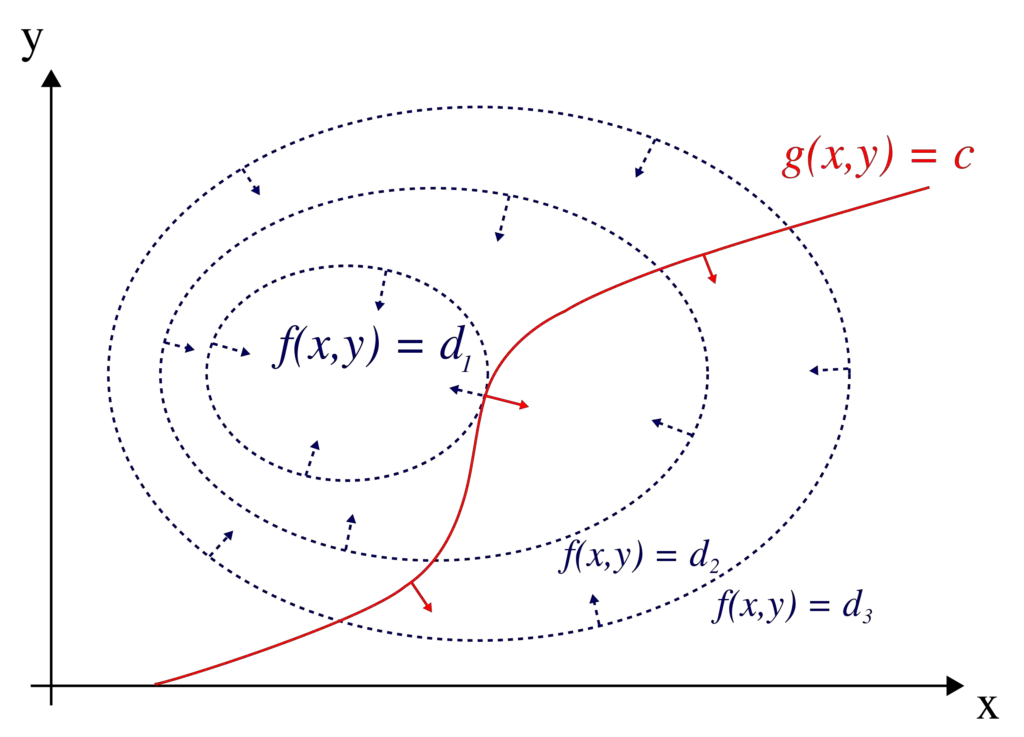
This means, we just have to multiply the gradient of f(x,y) by some scalar λ for it to equal the gradient of g(x,y).

Δg= λΔf

LaGrange Multipliers Example

Let’s say we have a function g(x,y) constrained by the circle f(x,y).

g(x,y) = x^2+y\\
f(x,y) = x^2+y^2=1 

First, we calculate the gradient of both functions.

Δg = \begin{bmatrix}
    2x \\
     1
  \end{bmatrix} \;
Δf = \begin{bmatrix}
    2x \\
     2y
  \end{bmatrix} \\

Next, we plug this into our Lagrange equality function.

\begin{bmatrix}
    2x \\
     1
  \end{bmatrix} = 
λ
 \begin{bmatrix}
    2x \\
     2y
  \end{bmatrix} \\

Solving the two functions, we obtain y and λ.

y = 0.5 \\ λ = 1

Now, we can plug this into our constraint equation f(x,y) = 1

x^2+y^2 = 1\\
x^2 = 0.75 \\
x = 0.87 \;or \; x = -0.87

Finally, we know our min and max.

min = \begin{bmatrix}
    0.75 \\
     -0.87
  \end{bmatrix} \;
max = \begin{bmatrix}
    0.75 \\
     0.87
  \end{bmatrix}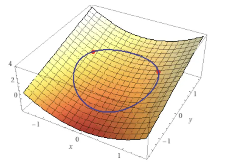 

This post is part of a series on Calculus for Machine Learning. To read the other posts, go to the index.