Covariance and Correlation

Int this post, we introduce covariance and correlation, discuss how they can be used to measure the relationship between random variables, and learn how to calculate them.
Covariance and Correlation are both measures that describe the relationship between two or more random variables.
What is Covariance
The formal definition of covariance describes it as a measure of joint variability. If one random variable X varies, does Y vary simultaneously, and if so, by how much and in what direction?
Accordingly, the covariance is primarily useful to determine relationships between variables.
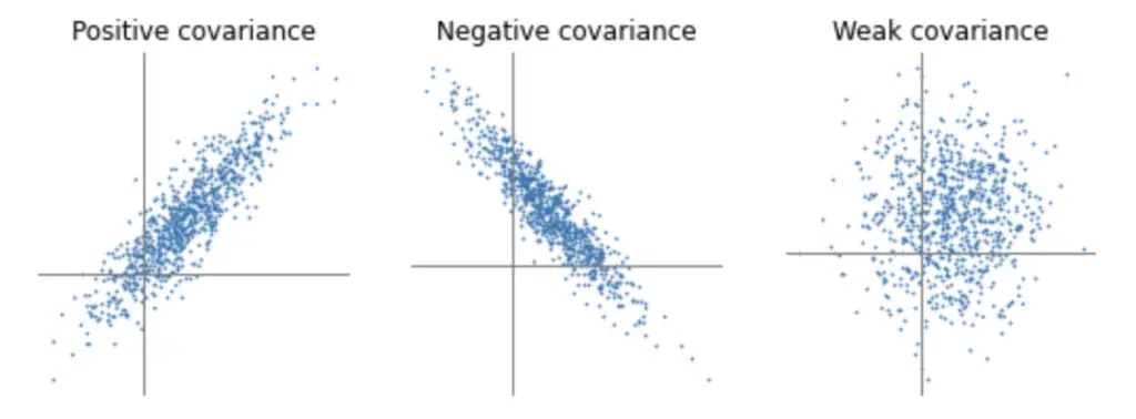
In the second plot, the covariance is clearly negative. As X increases, Y decreases.
In the last plot, the relationship is not as clear-cut.
Since we already know how to calculate the expected values of X and Y, we only need to take a small step to obtain the covariance formula. It is simply the expected value of X times Y minus the expected value of X times the expected value of Y.
Cov(X,Y) = E[XY] - E[X]E[Y]
This is a more succint form of the following expression.
Cov(X,Y) = E[(X-E[X])(Y-E[Y])]
Covariance for Discrete Random Variables
The general form introduced above can be applied to calculate the covariance of concrete random variables X and Y when (X, Y) can assume n possible states such as (x_1, y_1) are each state has the same probability.
Cov(X,Y) = \sum_{i=1}^n (x_i - E(X))(y_i-E(Y))Covariance for Continuous Random Variables
If X and Y are continuous random variables, the covariance can be calculated using integration where p(x,y) is the joint probability distribution over X and Y.
Cov(X,Y) = \int_{-\infty}^{\infty}(x-E(X))(y-E(Y)p(x,y)dxdyWhat is the Correlation Coefficient
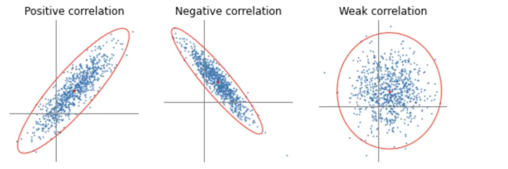
Closely related to the covariance is the correlation coefficient. While the covariance indicates the relationship of a variable, it doesn’t inform us about the magnitude of the relationship. This is where the correlation comes in. By calculating Pearson’s correlation coefficient, we not only have a measure of the direction but also of the magnitude of the relationship between two random variables X and Y.
Given the covariance, the formula for the correlation coefficient is fairly simple. You need to divide the covariance by the product of the standard deviations of X and Y. Remember that the standard deviation is just the square root of the variance.
Cor(X, Y) = \frac{Cov(X,Y) }{\sqrt{Var(X)Var(Y)}} = \frac{Cov(X,Y) }{\sigma_X\sigma_Y}Dividing by the product of the standard deviations normalizes the covariance so that the correlation coefficient assumes a unitless value between -1 and 1.
- The closer the correlation coefficient to one the stronger the positive correlation.
- The closer the correlation coefficient to minus one the stronger the negative correlation.
- The closer the correlation coefficient zero the weaker the correlation.
I won’t go through a manual step by step example like I did in the post about variance and expected values, because it’s basically just a repetition of that process. Since you have a joint probability distribution p(x,y) over 2 variables, you would have to
- calculate the expected value and variance of the marginal mass or density function with respect to X to get E[X] and Var[X].
- calculate the expected value and variance of the marginal mass or density function with respect to Y to get E[Y] and Var[Y].
- calculate the expected value of the joint mass or density function to obtain E[XY].
- Plug these values into the formulae for the covariance and correlation
It won’t help your conceptual understanding very much if we grind through an example and you’ll probably never have to do it by hand.
However, if you still want to go through a step by step example, here is a worksheet from Imperial College.
Covariance Matrix
So far we’ve only calculated the covariance and variance between 1-dimensional variables, which results in single number outcomes.
For higher-dimensional data, the variance and covariance can be succinctly captured in a variance-covariance matrix also known as the covariance matrix. Given two variables x, and y the covariance matrix would look like this.
\begin{bmatrix}
cov(x,x) && cov(x,y) \\
cov(y,x) && cov(y,y)
\end{bmatrix}
=
\begin{bmatrix}
var(x) && cov(x,y) \\
cov(y,x) && var(y)
\end{bmatrix}
Notice that the main diagonal contains the variances of x and y. The covariance of a variable with itself is its variance.
Furthermore, covariance operations are commutative. Accordingly, cov(x,y) and cov(y,x) are equivalent. This also implies that the variance-covariance matrix is symmetric across its main diagonal.
This covariance matrix can be constructed for vectors of any number of dimensions. If you have a random variable X with x_n states.
x= \begin{bmatrix}
x_1 \\
x_2\\
...\\
x_n
\end{bmatrix}
the calculation of the covariance can be expressed as a matrix operation.
Cov(X,X) = E[(X-E[X])(X-E[X])^T] \\
=E[XX^T] - E[X]E[X^T]
The result is a covariance matrix of the following form.
\begin{bmatrix}
cov(x_1,x_1) &&  ... && cov(x_1,x_n)\\
...\\
cov(x_n,x_1) && ... && cov(x_n,x_n)
\end{bmatrix}
This post is part of a series on statistics for machine learning and data science. To read other posts in this series, go to the index.
