Gram Schmidt Process: A Brief Explanation

The Gram Schmidt process is used to transform a set of linearly independent vectors into a set of orthonormal vectors forming an orthonormal basis. It allows us to check whether vectors in a set are linearly independent.

In this post, we understand how the Gram Schmidt process works and learn how to use it to create an orthonormal basis.

What is the use of Gram Schmidt?

We’ve established previously that the identity matrix of an orthogonal matrix can be obtained by simply transposing it. So we don’t have to go through complicated linear transformations to obtain the identity.

Furthermore, the projection of a vector b into an orthonormal basis is much easier because you only have to take the dot product of b with all the basis vectors of the orthonormal basis.

Introducing the Simplified Projection Matrix

If you wanted to project any vector b into any vector space in which the basis vectors form the matrix A, you would have to perform the following transformation.

proj_vb = A(A^{T}A)^{-1}A^Tb

So your projection matrix is represented by this convoluted term

P = A(A^{T}A)^{-1}A^T

If you are interested in how we arrived at this expression, I’d suggest you check out the following explanation from MIT Open Courseware.

Applying this transformation is a laborious process not only for humans but also for computers. We have to do lots of matrix multiplications and transformations. Finding the inverse is especially time-consuming.
If A is an orthogonal matrix, that is, the basis vectors of our vector space form an orthonormal basis, the projection matrix can be simplified.

Remember that in an orthogonal matrix, the following rule applies.

A^T =A^{−1} \, therefore \, A^TA = I

Accordingly, our transformation matrix simplifies to

P = A(I)^{-1}A^T = AIA^T = AA^T

How the Gram Schmidt Process Works

Suppose we have a linearly independent set of vectors V={v1, v2, …vn}.
Our vectors in V all lie inside some vector space. We now need to find a set of vectors {q1, q2,…qn} that are orthogonal and of unit length, which span this vector space. We already know how to get to a vector of unit length. We simply divide by the vector’s length. For the first vector q1, we don’t need to worry about orthogonality since we haven’t discovered the other vectors q2, etc., yet. So to get from v1 to q1, we simply perform the following.

q_1 = \frac{v_1}{|v_1|}

Now we need to find the vector q2, which is of unit length and orthogonal to q1. Furthermore, q2 needs to lie in the plane spanned by v1 and v2. If it didn’t lie in the plane, it wouldn’t form a basis for the same vector space inhabited by v1 and v2.

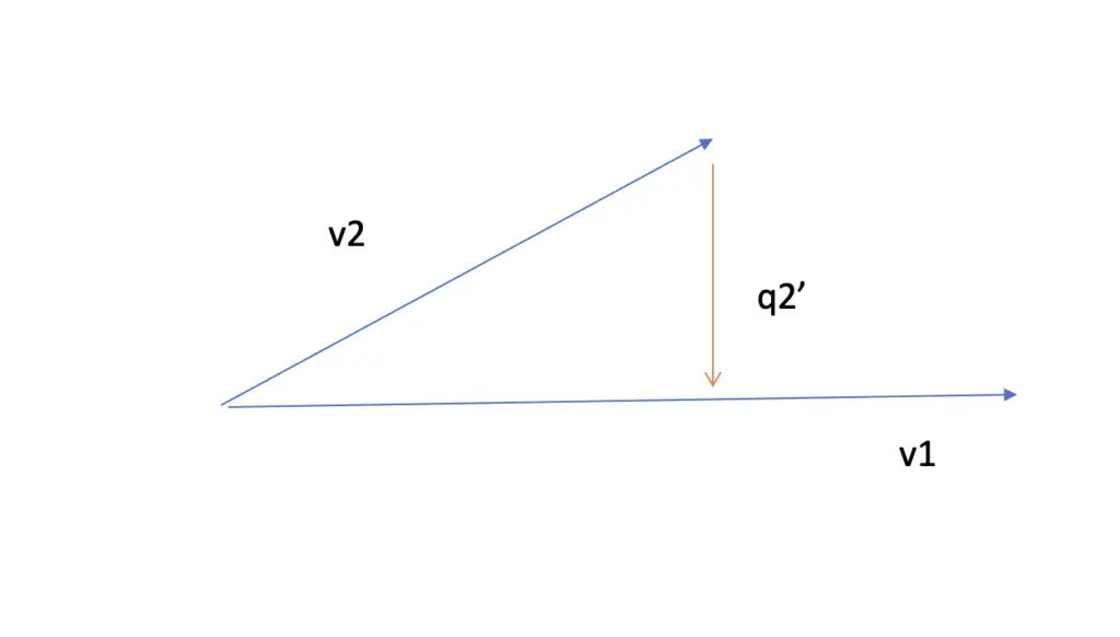
In the chapter on vector projections, we discussed how to obtain the projection of v2 onto v1. Using the unit vector of v1, which is q1, we arrive at this expression.

proj_{v1}v2 = \frac{q_1 \cdot v_2}{|q_1|^2}q_1 = (q_1 \cdot v_2)q_1 

Note that |q1| is just 1, so we can eliminate it.

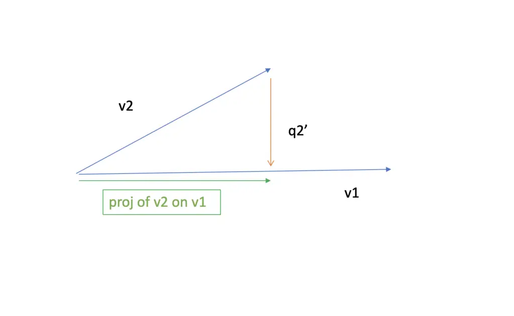
Now, to get to q2, we obtain the difference between v2 and the projection of v2 on v1.

q_2' = v_2 - (v_2 \cdot q_1)q_1 

and then obtain the unit vector.

q_2 = \frac{q_2'}{|q_2'|}

To find q3, we’d have to find a vector that is orthogonal to q1 and q2. Accordingly, we need to perform the following operations.

q_3' = v_3 - (v_3 \cdot q_1)q_1 -  (v_3 \cdot q_2)q_2

q_3 = \frac{q_3'}{|q_3'|}

We can formalize this process as follows.

q_n' = v_n - \sum_{i=1}^{n-1}(v_n \cdot q_i)q_i \,and\, q_n=\frac{q_n'}{|q_n'|}

Example

v_1 = \begin{bmatrix}
    1 \\
    1 \\
    0 \\
  \end{bmatrix}
v_2 = \begin{bmatrix}
    1 \\
    0 \\
    1 \\
  \end{bmatrix}

q_1 = 
\frac{v1}{|v_1|} = 
\frac{1}{\sqrt(2)} 
\begin{bmatrix}
    1 \\
    1 \\
    0 \\
  \end{bmatrix}

q_2' = v_2 - (v_2 \cdot q_1)q_1  =
\begin{bmatrix}
    1 \\
    0 \\
    1 \\
  \end{bmatrix}
-
(\begin{bmatrix}
    1 \\
    0 \\
    1 \\
  \end{bmatrix}
\frac{1}{\sqrt(2)} 
\begin{bmatrix}
    1 \\
    1 \\
    0 \\
  \end{bmatrix})
\frac{1}{\sqrt(2)} 
\begin{bmatrix}
    1 \\
    1 \\
    0 \\
  \end{bmatrix}

q_2' = 
\begin{bmatrix}
    1 \\
    0 \\
    1 \\
  \end{bmatrix}
-
1
\begin{bmatrix}
    1 \\
    1 \\
    0 \\
  \end{bmatrix}
=
\begin{bmatrix}
    1 \\
    -1 \\
    0 \\
  \end{bmatrix}

q_2 = 
 
\frac{1}{\sqrt(2)} 
\begin{bmatrix}
    1 \\
    -1 \\
    0 \\
  \end{bmatrix}

You can make sure that q1 and q2 truly are orthonormal vectors by checking that the dot product of q1 and q2 is zero and that their respective lengths are 1.

This post is part of a series on linear algebra for machine learning. To read other posts in this series, go to the index.