What is Linear Independence: An Explanation by Example

In this post we define linear independence and walk through an example to develop an intuitive understanding of the concept.

What is Linear Independence?

When a set of several vectors is linearly independent, it is not possible to represent one vector as a linear combination of the remaining vectors in the set. Two orthogonal vectors are linearly independent.

What is a Linear Combination?

A linear combination is a vector that is created by combining two or more vectors through addition or subtraction. The constituent vectors can be scaled by arbitrary numbers. The vector v3 is a linear combination of v1 and v2 if it can be expressed in the following form where a and b are scalar numbers.

v_3 = av_1 + bv_2 

Understanding Linear independence by Example

Now you might be wondering what’s the use of learning all these obscure vector operations like the dot product. Here is a little primer.
As we established in the introduction, vectors can be used to represent data across multiple dimensions. Now individual data attributes or features might be correlated, or they might be completely independent of each other. 

Imagine you had a bakery, and you had to model the price of donuts, the price of bread, and the price of bagels.
The prices are determined by a variety of factors such as the price of dough, cost of labor to pay your employees, etc. These affect donuts, bread, and bagels since all require dough and a baker to make them. 

Your price of these items would increase if the cost of labor or the cost of dough were to increase. But they may not increase by the same magnitude. A donut or a bagel probably requires less dough than one bread, so an increase in the price of dough would increase the price of bread by a larger margin.
Let’s just assume a donut costs 1 unit of dough and 2 units of labor. A bread costs 2 units of dough and 3 units of labor, and a bagel 1 unit of dough and 1 unit of labor.

donut \, price =
\begin{bmatrix}doughcost\\labor cost\end{bmatrix}
=
\begin{bmatrix}1\\2\end{bmatrix} 

bread \, price =
\begin{bmatrix}doughcost\\labor cost\end{bmatrix}=
\begin{bmatrix}2\\3\end{bmatrix}

bagel \, price =
\begin{bmatrix}doughcost\\labor cost\end{bmatrix}
=
\begin{bmatrix}1\\1\end{bmatrix}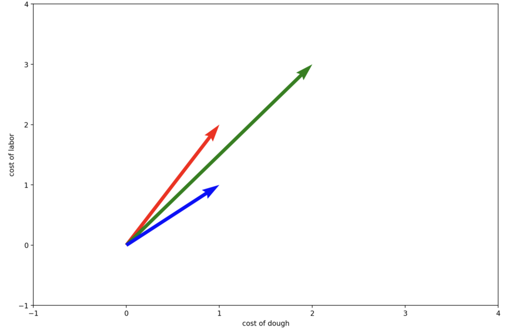 

red = price of one bread

green = price of one donut

blue = price of one bagel

Since both are affected by the costs of labor and dough, the prices of donuts and bread are clearly correlated.

Let’s assume some bakers have gone off doing some crazy baking experiments like pizza that has caused the company a loss. Accordingly, overly close-minded management has imposed a rule that bakers can only use dough and labor in the specific combinations of quantities required by these three products. So you can either use 1 unit of dough with 2 units of labor, 2 units of dough with 3 units of labor, or 1 unit of dough with 1 unit of labor. Bakers are free to combine resources from two products to create a third product. For example, they can use the resources for a donut and a bagel to make one bread.

\begin{bmatrix}1\\2\end{bmatrix} 
+
\begin{bmatrix}1\\1\end{bmatrix} 
=
\begin{bmatrix}2\\3\end{bmatrix} 

The fact that this is possible and we can create one of the vectors as a combination of the others is known as linear dependence in linear algebra terms.

Let’s assume management decides to kill bagels and the corresponding resource combination from production.

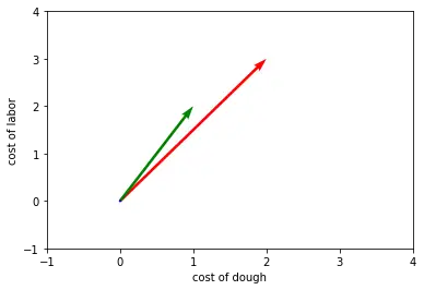
Now, we are left with only donuts and bread. Now it is no longer possible to combine the set of resources of one product to create another one. We could try to take the resources from two donuts, but that would not result in the exact amount of resources to make one or several loaves of bread.

\begin{bmatrix}1\\2\end{bmatrix} 
+
\begin{bmatrix}1\\2\end{bmatrix} 
\neq
\begin{bmatrix}2\\3\end{bmatrix} 

In linear algebra terms, we would say the two vectors are linearly independent.

But surely there are different requirements for making donuts that do not affect bread and vice versa. For example, a donut may have chocolate glazing, while a bread needs sunflower seeds.
For the sake of simplicity let’s just assume the price of bread is entirely dependent on  the price of sunflower seeds and the cost of a donut only depends on the cost of chocolate:

donut \, price =
\begin{bmatrix}chocolatecost\\sunflowerseedcost\end{bmatrix}
=
\begin{bmatrix}1\\0\end{bmatrix}

bread\,price
=
\begin{bmatrix}chocolatecost\\sunflowerseedcost\end{bmatrix}
=
\begin{bmatrix}0\\3\end{bmatrix}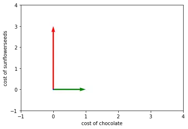

red = price of one bread

green = price of one donut

Did you spot anything? Exactly, now the two vectors are orthogonal to each other, because the prices of donuts and bread are determined by completely independent features. The price of chocolate does not affect the price of bread and the price of sunflower seeds does not affect the price of donuts.

We can prove this mathematically by determining that the dot product equals zero.

donut \cdot bread = \begin{bmatrix}1\\0\end{bmatrix}
\cdot
\begin{bmatrix}0\\3\end{bmatrix}
=
1 \times 0 + 0\times 3 = 0

Now, the price of donuts is not only linearly independent of the price of bread but the prices are also no longer correlated. Changes in the price of resources of bread do not affect the price of donuts at all.

For machine learning, this has huge implications because machine learning models attempt to find patterns in data and relationships between features to make predictions.

In the first case data indicating an increase in the price of bread would probably lead a machine learning model to also predict an increase in the price of donuts. Because thanks to linear algebra the model knows that the two prices are highly correlated.

In the second case it should not predict an increase in donut price based on increases in the price of bread because the two are not related.

Another useful implication is the curse of dimensionality.

Here we just looked at two dimensions, but machine learning models usually deal with thousands or millions of features, meaning they have to perform calculations across millions of dimensions. Every additional dimension increases the computational load exponentially.
If we can find highly correlated features, it might be reasonable to merge them into one feature to reduce the data dimension, although this might come at the cost of model performance. As a machine learning practitioner, you might have to face a trade-off between computational efficiency and model performance.

To understand how these feature reduction techniques work, we have to learn about vector projections.

Summary

Two vectors are linearly independent if the dot product between them equals zero. However, a zero-valued dot product is not sufficient to determine linear independence.

This post is part of a series on linear algebra for machine learning. To read other posts in this series, go to the index.