Understanding Hinge Loss and the SVM Cost Function

In this post, we develop an understanding of the hinge loss and how it is used in the cost function of support vector machines.

Hinge Loss

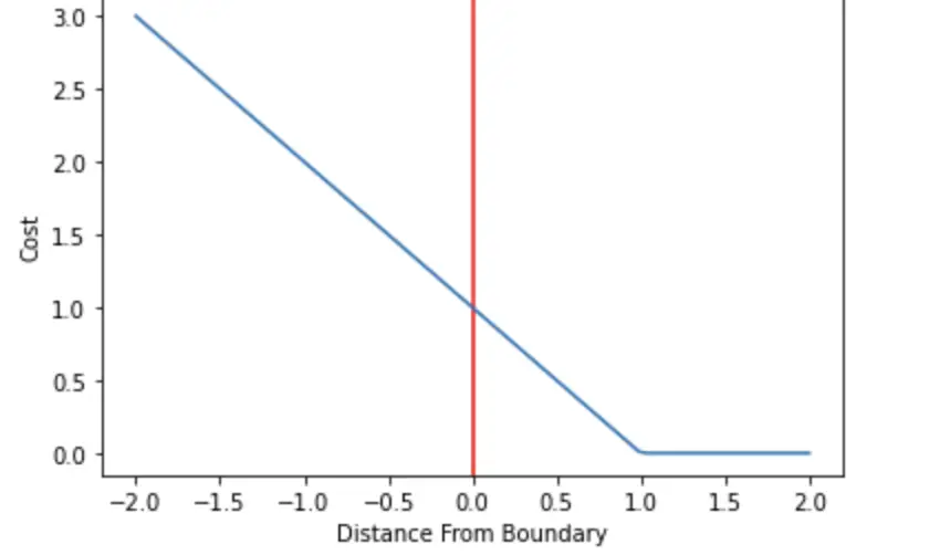
The hinge loss is a specific type of cost function that incorporates a margin or distance from the classification boundary into the cost calculation. Even if new observations are classified correctly, they can incur a penalty if the margin from the decision boundary is not large enough. The hinge loss increases linearly.

The hinge loss is mostly associated with soft-margin support vector machines.

If you are familiar with the construction of hyperplanes and their margins in support vector machines, you probably know that margins are often defined as having a distance equal to 1 from the data-separating-hyperplane. Otherwise, check out my post on support vector machines (link opens in new tab), where I explain the details of maximum margins classifiers. We want data points to not only fall on the correct side of the hyperplane but also to be located beyond the margin.

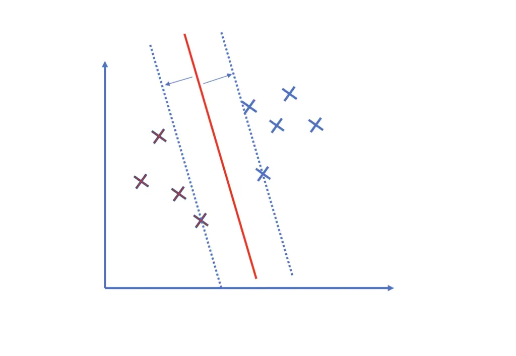
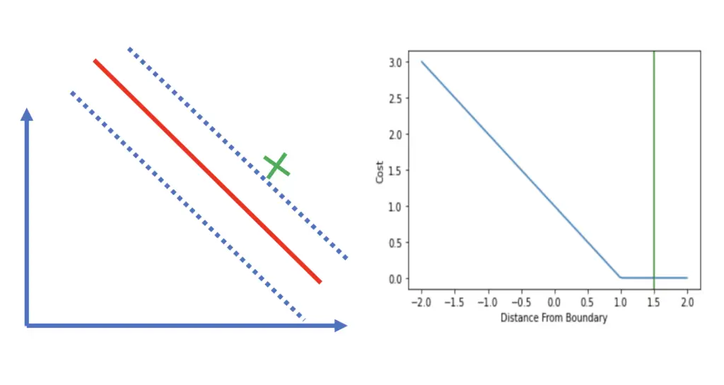
Support vector machines address a classification problem where observations either have an outcome of +1 or -1. The support vector machine produces a real-valued output that is negative or positive depending on which side of the decision boundary it falls. Only if an observation is classified correctly and the distance from the plane is larger than the margin will it incur no penalty. The distance from the hyperplane can be regarded as a measure of confidence. The further an observation lies from the plane, the more confident it is in the classification.
For example, if an observation was associated with an actual outcome of +1, and the SVM produced an output of 1.5, the loss would equal 0.

Contrary to methods like linear regression, where we try to find a line that minimizes the distance from the data points, an SVM tries to maximize the distance. If you are interested, check out my post on constructing regression lines. Comparing the two approaches nicely illustrates the difference between the nature of regression and classification problems.

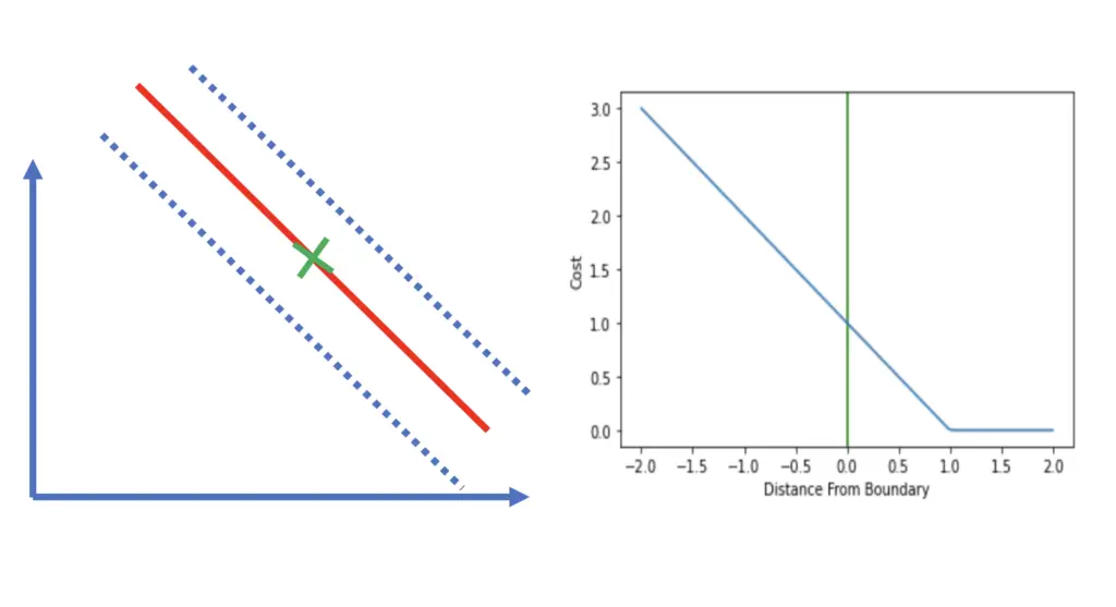
An observation that is located directly on the boundary would incur a loss of 1 regardless of whether the real outcome was +1 or -1.

Observations that fall on the correct side of the decision boundary (hyperplane) but are within the margin incur a cost between 0 and 1.

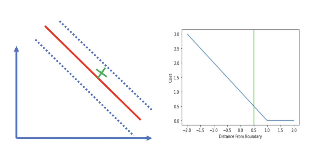
All observations that end up on the wrong side of the hyperplane will incur a loss that is greater than 1 and increases linearly. If the actual outcome was 1 and the classifier predicted 0.5, the corresponding loss would be 0.5 even though the classification is correct.

Now that we have a strong intuitive understanding of the hinge loss, understanding the math will be a breeze.

HInge Loss Formula

The loss is defined according to the following formula, where t is the actual outcome (either 1 or -1), and y is the output of the classifier.

l(y) = max(0, 1 -t \cdot y)

Let’s plug in the values from our last example. The outcome was 1, and the prediction was 0.5.

l(y) = max(0, 1 - 1 \cdot 0.5) = 0.5

If, on the other hand, the outcome was -1, the loss would be higher since we’ve misclassified our example.

l(y) = max(0, 1 - (-1) \cdot 0.5) = 1.5

Instead of using a labelling convention of -1, and 1 we could also use 0 and 1 and use the formula for cross-entropy to set one of the terms equal to zero. But the math checks out more beautifully in the former case.

With the hinge loss defined, we are now in a position to understand the loss function for the support vector machine. But before we do this, we’ll briefly discuss why and when we actually need a cost function.

Hard Margin vs Soft Margin Support Vector Machine

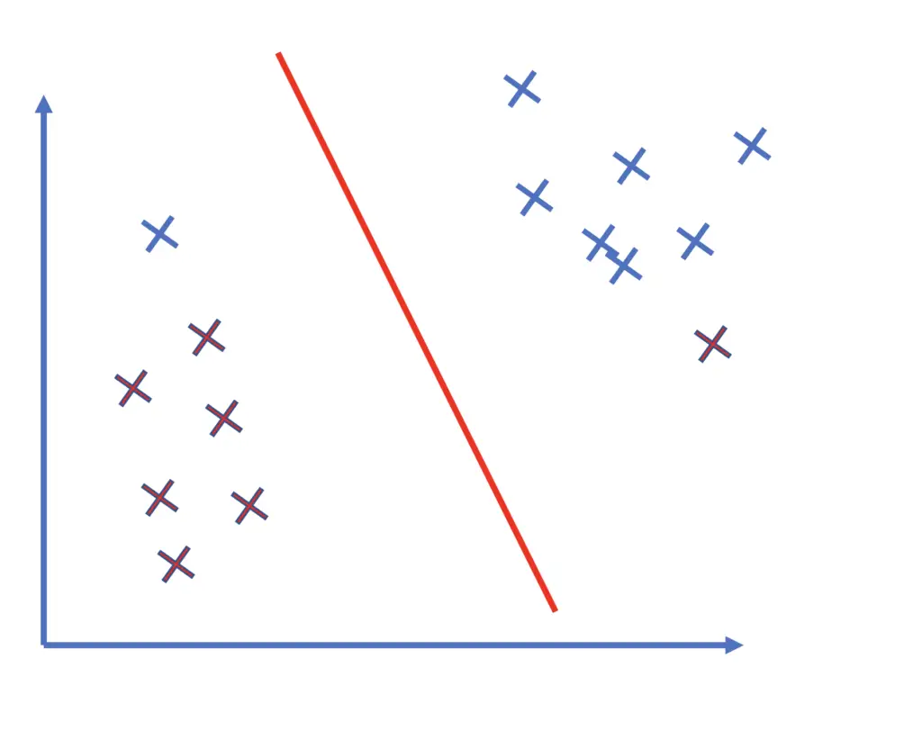
In a hard margin SVM, we want to linearly separate the data without misclassification. This implies that the data actually has to be linearly separable.

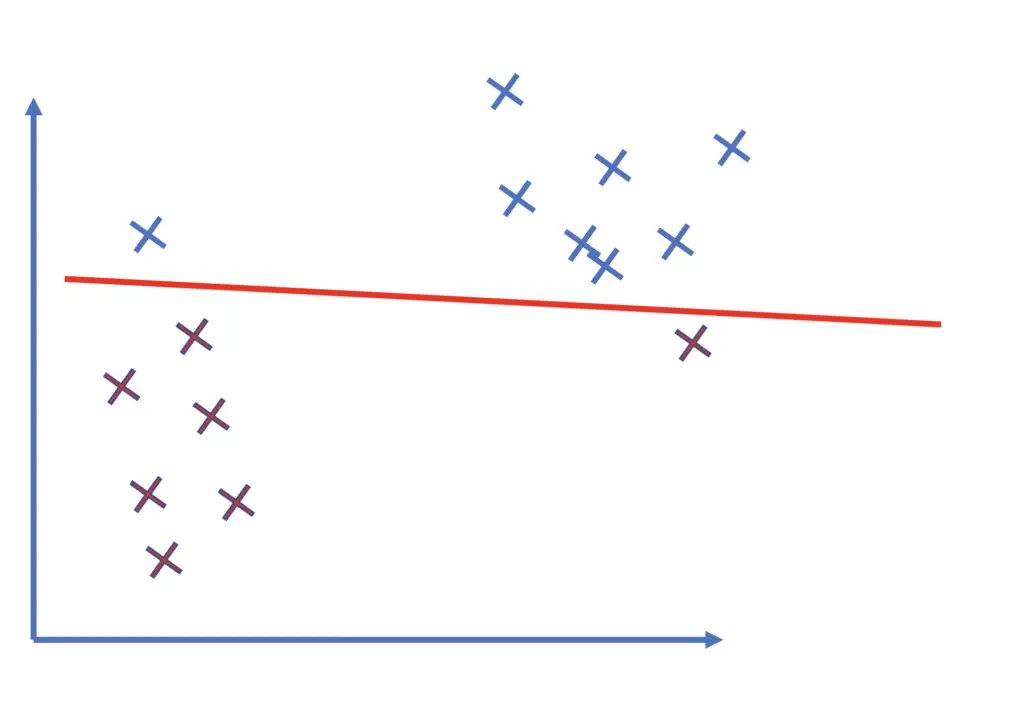
If the data is not linearly separable, hard margin classification is not applicable.
Even though support vector machines are linear classifiers, they are still able to separate data points that are not linearly separable by applying the kernel trick. To understand how kernels work, check out my post on kernels in machine learning (link opens in new tab).

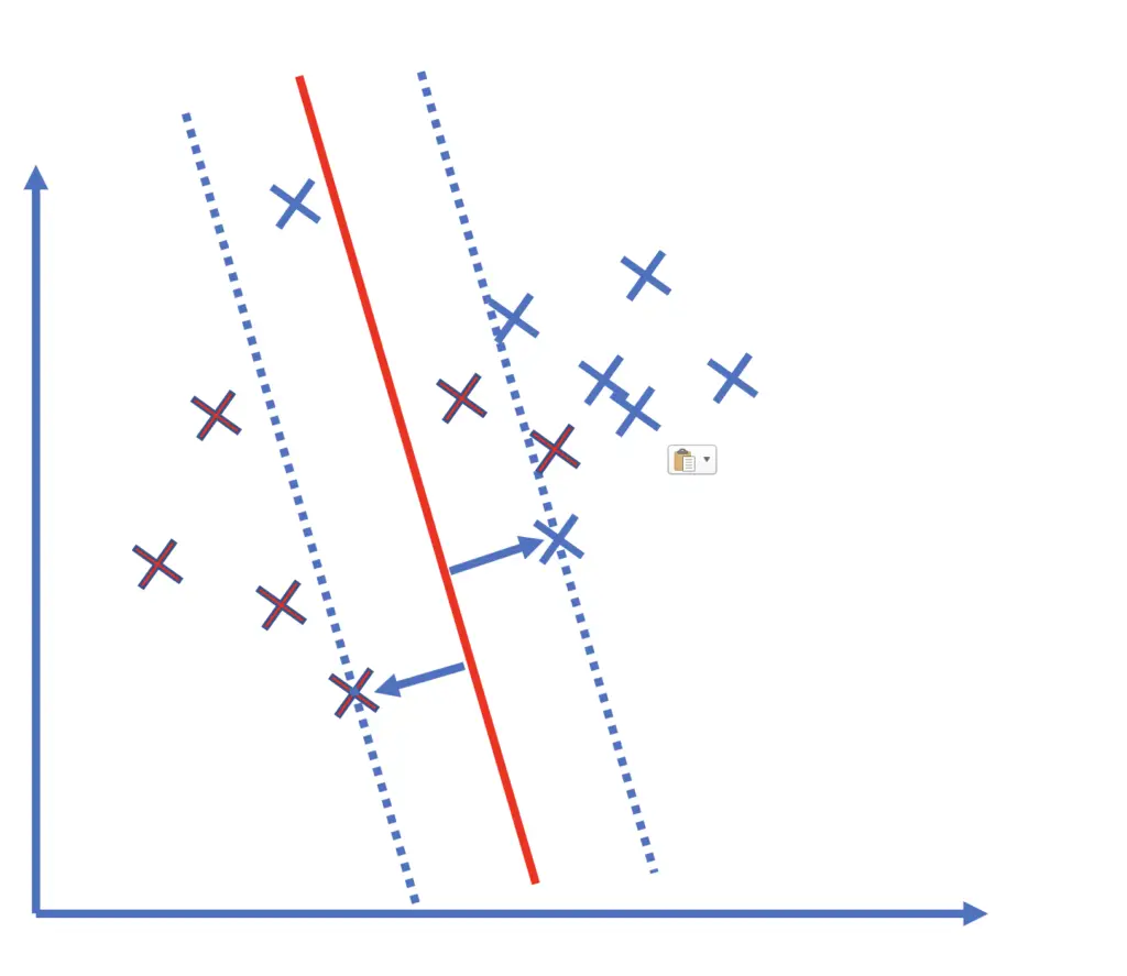
Furthermore, if the margin of the SVM is very small, the model is more likely to overfit. In these cases, we can choose to cut the model some slack by allowing for misclassifications. We call this a soft margin support vector machine. But if the model produces too many misclassifications, its utility declines. Therefore, we need to penalize the misclassified samples by introducing a cost function.

In summary, the soft margin support vector machine requires a cost function while the hard margin SVM does not.

SVM Cost

In the post on support vectors, we’ve established that the optimization objective of the support vector classifier is to minimize the term w, which is a vector orthogonal to the data-separating hyperplane onto which we project our data points.

\min_{w} \frac{1}{2} \sum^n_{i=1}w_i^2

This minimization problem represents the primal form of the hard margin SVM, which doesn’t account for classification errors.

For the soft-margin SVM, we combine the minimization objective with a loss function such as the hinge loss.

\min_{w} \frac{1}{2} \sum^n_{i=1}w_i^2 + \sum^m_{j=1} max(0, 1 -t_j \cdot y_j)

The first term sums over the number of features (n), while the second term sums over the number of samples in the data (m).
The t variable is the output produced by the model as a product of the weight parameter w and the data input x.

t_i = w^Tx_j

To understand how the model generates this output, refer to the post on support vectors (link opens in new tab).

The loss term has a regularizing effect on the model. But how can we control the regularization? That is how can we control how aggressively the model should try to avoid misclassifications. To manually control the number of misclassifications during training, we introduce an additional parameter, C, which we multiply with the loss term.

\min_{w} \frac{1}{2} \sum^n_{i=1}w_i^2 + C\sum^m_{j=1} max(0, 1 -t_j \cdot y_j)

The smaller C is, the stronger the regularization. Accordingly, the model will attempt to maximize the margin and be more tolerant towards misclassifications.

If we set C to a large number, then the SVM will pursue outliers more aggressively, which potentially comes at the cost of a smaller margin and may lead to overfitting on the training data. The classifier might be less robust on unseen data.

Summary

The hinge loss is a special type of cost function that not only penalizes misclassified samples but also correctly classified ones that are within a defined margin from the decision boundary.

The hinge loss function is most commonly employed to regularize soft margin support vector machines. The degree of regularization determines how aggressively the classifier tries to prevent misclassifications and can be controlled with an additional parameter C. Hard margin SVMs do not allow for misclassifications and do not require regularization.

For some hands-on practice, Coursera offers a nice guided programming project on building SVMs from scratch (link opens in new tab).

This post is part of a larger series I’ve written on machine learning and deep learning. For a comprehensive introduction to deep learning, check out my blog post series on neural networks. My series on statistical machine learning techniques covers techniques such as linear and logistic regression.