Types of Machine Learning: A High-Level Introduction

In machine learning, we distinguish between several types and subtypes of learning and several learning techniques.

Broadly speaking, machine learning comprises supervised learning, unsupervised learning, and reinforcement learning. Problems that do not fall neatly into one of these categories can often be classified as semi-supervised learning, self-supervised learning, or multi-instance learning. In supervised learning, we generally distinguish between regression and classification problems.

Regression vs Classification

Supervised learning tasks involve either a regression problem or classification problem.

In a regression scenario, the model attempts to predict a continuous numerical output. An example is predicting the price of a house. If your model returns an exact dollar value, you have a regression model.

A classification problem involves classifying examples into groups. We could train a housing price model to classify houses into one of several pricing groups. In that case, we are dealing with a classification problem.

For beginners, the difference between the two approaches may not always be as clear-cut.

Besides the difference in the predicted output, the two approaches are similar with regard to the predictors. The predictors can have real or discrete values.
Classification models often return a class probability, a continuous output, rather than a class label. Outcomes are sorted into the class with the highest associated probability returned by the model.
Regression models may predict integer values that could also be interpreted as classes. For example, a housing price model that returns a dollar-accurate price could be interpreted as a classification model in which every possible price is a class.

For evaluating the predictive performance of a model, the distinctions matter, though. Regression models are evaluated differently from classification models.

Evaluating Classification Models

To evaluate a classification model, accuracy is the most commonly used measure. Accuracy is fairly straightforward to calculate since it is just the percentage of the total examples that have been classified correctly. If 800 out of 1000 samples have been classified correctly, your accuracy is 80%
In a binary classification problem such as “Does the patient have a certain disease or not” you would add up the number of patients that have been classified as having the disease and actually have the disease (true positives) and the number of patients that have been classified as not having the disease and that really do not have the disease (true positives). Their percentage of the total number of evaluated cases makes up the accuracy. This result can be visualized in a confusion matrix.

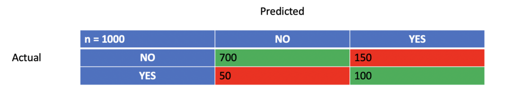
So your accuracy is:

\frac{True Positive + TrueNegative}{Total} = \frac{700 + 100}{1000} = 0.8 = 80\%

Accuracy is a crude measure that is often not enough. In man classification scenarios, you are interested in more granular results. For example, if your model is used to predict whether a tumor is malignant or benign, you would care much more about reducing false negatives than false positives. In the second case, the patient might get a shock, but actually, there is no reason to worry. A follow-up test will likely identify her as not having cancer. If you tell a patient who has cancer that she is healthy, you may very well cause premature death. You want your model to have high sensitivity (the ability to identify true positives correctly).

In our case, the sensitivity is calculated as follows:

Sensitivity = \frac{TruePositive}{TruePositive+FalseNegative} 

= \frac{100}{100 + 50} = 0.667 = 67%

I wouldn’t use this model to classify diseases, given this sensitivity.

In other scenarios, you are more interested in the specificity (the ability to identify true negatives correctly). In a legal context, most people would probably agree that false positives (punishing an innocent person) are worse than false negatives (letting a guilty person walk free). You can calculate the specificity as follows:

Specificity = \frac{TrueNegative}{FalsePositive+TrueNegative} 

= \frac{700}{700 + 150} = 0.82 = 82%

The confusion matrix can be extended to cases with more than two classes.

Evaluating Regression Models

Since a regression model predicts a continuous numerical output, you need a more advanced mathematical measure to quantify the error in the prediction. A simple percentage value like accuracy is not enough. The most common measure is the root mean squared error (RMSE). The RMSE measures the average deviation of the predicted value from the actual value and sums up these differences across the entire training set.

RMSE = \sqrt{\frac{\sum_{i=1}^N(actual_i - predicted_i)^2}{N}}

Squaring the difference helps in two ways. Firstly, it ensures that all measures are positive. Secondly, it punishes large differences disproportionately more than smaller ones.

Let’s say we have a regression model, and we feed it two values. The actual values are 5 and 6.2, and the model predicts 4.5 and 6, respectively. We can calculate the RMSE as follows:

RMSE = \sqrt{\frac{(5 - 4.5)^2+(6.2-6)^2}{2}} = 0.38

Supervised vs Unsupervised Learning

If you train a model on a dataset that consists of predictors and corresponding target variables, you are generally dealing with a supervised learning problem. The model is trained to learn a mapping from the predictors to the target output.

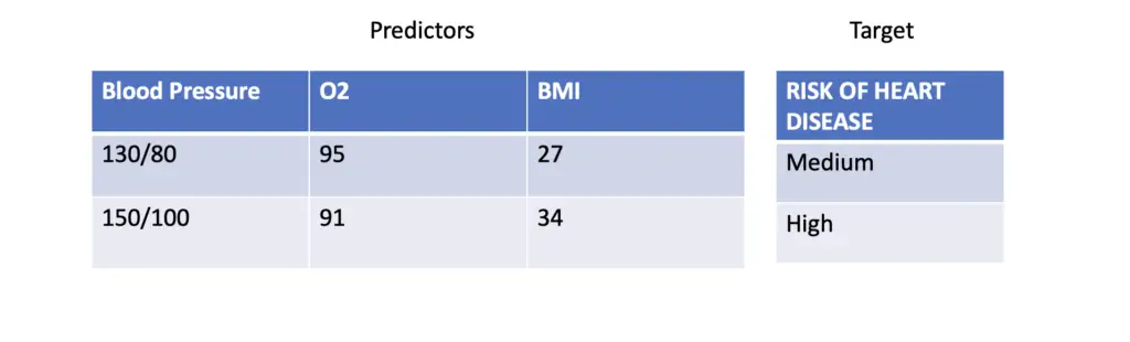
For example, using average blood pressure, average oxygen saturation, and body mass index to predict the risk of heart disease would be a supervised learning problem.

Examples of supervised learning algorithms are linear regression, logistic regression, decision trees, and support vector machines.

In an unsupervised learning problem, you would use a model to discover patterns in the data without predicting a certain target value. If you do not yet have a risk classification system for heart disease and reliable data for what constitutes a certain risk level, you could use an unsupervised learning model on the predictors. For example, people with a high BMI might have lower blood oxygen levels. Using a technique called clustering, you can find out whether the data points form groups. For example, let’s say people with a BMI around 34 in your sample also have O2 measurements around 91.

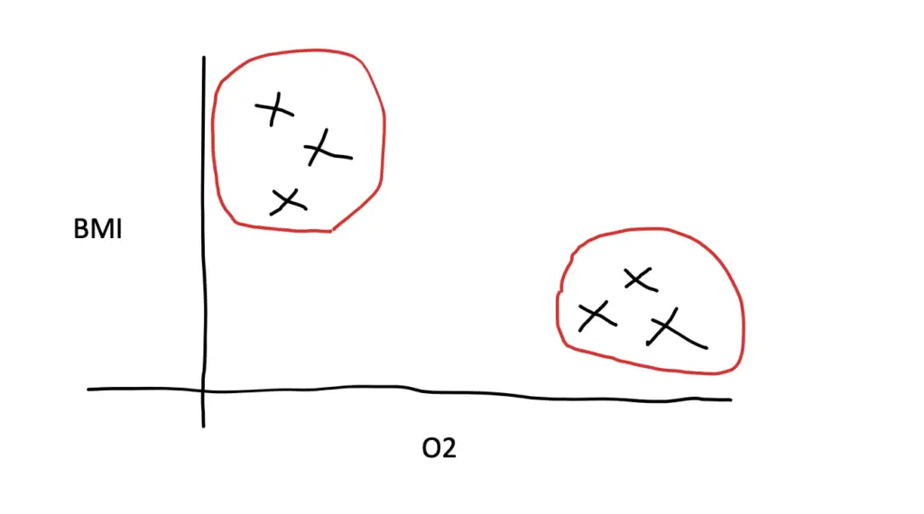
Now you can zoom in on that particular group and see whether they have a higher prevalence of heart disease than the other groups.
Supervised learning is often concerned with making the data easier to understand and interpret. In addition to
clustering, density estimation, and dimensionality reduction techniques such as principal components analysis are commonly used to better understand the data.

Typical examples for unsupervised machine learning algorithms are K-means clustering or K-nearest neighbors.

The essential difference between supervised and unsupervised learning is that you have a target variable in supervised learning situations. This implies that you need sufficiently large size of samples where you already know the outcome. In problems like image recognition, this also means that your samples need to be labeled with the outcome of the target variable. If you want to use an image to train a model to recognize cats, the image needs to be labeled with the information of whether it actually contains a cat or not.

Ensemble Learning

Ensemble learning combines multiple learning algorithms to attain better overall performance. The basic premise is that greater diversity among models will lead to a better overall predictive performance since each model will pick up aánd emphasize a different aspect of the learning problem. The diversity can be achieved by either combining completely different types of models, known as hybrid ensembles, or by ensuring diversity in the training process among otherwise similar models. You can train each model in an ensemble on a different subset of the training data or on a different subset of features.

Semi-Supervised Learning and Self-Supervised Learning

Some machine learning methods, especially those found in deep learning, cannot be neatly categorized as supervised or unsupervised.

Self-Supervised Learning

A general adversarial network is an unsupervised neural network used to create and synthesize new data. You feed it random input data, and it learns to create images or other types of structured data. But how does it learn to map from random noise to an image? You use another network trained to recognize images and constantly give feedback to the first network on how much its output resembles the desired image.
So you are essentially using a trained network to train an untrained network. This is known as a self-supervised learning problem.

Autoencoders operate according to a similar principle. They are trained to create a different representation of data called an encoding. This technique is beneficial for dimensionality reduction because the encoding is usually lower-dimensional and more information-efficient. But for the encoding to be useful, it has to be possible to reconstruct the original data representation from the decoded version. During training, the autoencoder consists of an encoder and a decoder. The encoder is tasked with encoding the data while the decoder takes the output of the encoder and attempts to reconstruct the original data. Thus, the input data is also the target data. Once the encoder has learned to create a satisfactory encoding, the decoder is no longer necessary.

In both of these cases, you are basically turning an unsupervised problem into a supervised one.

Semi-Supervised Learning

Semi-Supervised learning is often applied in scenarios where such large amounts of labeled data are required that creating a corpus of labeled data of the appropriate size is often not feasible. Machine translation and speech recognition are prime examples. When translating from one language to another or recognizing the human voice, the model has to deal with the enormous complexity and variability in human language. In addition to the semantics and syntax of the core language, people use their own dialects, abbreviations, and informal ways of communicating. Often, there doesn’t even exist training data for a certain regional dialect.
To tackle this problem, you can train a model on a few thousand or hundreds of thousands of labeled training examples such as sentence pairs. The patterns detected while learning the labeled representations can then be used to transfer knowledge to unlabelled data. For example, you might share sentence-level representations and lexical patterns detected in the training examples to make sense of input in dialects.

Reinforcement Learning

Reinforcement Learning is at the heart of modern robotics and currently represents the paradigm most closely associated with truly thinking machines and artificial general intelligence. The basic idea is to get a machine to independently learn to perform actions in a given situation by rewarding and penalizing it based on the chosen behavior. The agent’s goal is to maximize the reward defined by a function. Rather than being trained directly on given data, the agent attempts to optimize the reward function based on a process of trial and error. When interacting with its environment, the agent progresses through a series of states that are each associated with choices and rewards. Rewards a cumulative, and so the agent learns to treat all states as connected.
This way, you can get a robot to do a series of complex movements such as locating an item, picking it up, and carrying it to a certain location.

An AI agent can also apply reinforcement learning to learn a complex series of optimal moves in a board game. Alpha Go, the AI system that beat the reigning human champion at the game of Go in 2017, is based on reinforcement learning.
The superhuman performance was achieved by letting the algorithm play millions of games against itself.
During the training process, the agent alternates between exploration phases, where it tries new moves, and exploitation phases, where it actually makes the moves it has determined to be ideal in the exploration phase.

That way, Alpha Go learned to optimize series of movements over longer and longer sequences of moves. Ultimately, whenever its opponent made a move, Alpha Go was able to immediately map out the next several moves and all their associated cumulative probabilities of leading to victory.

The biggest challenge associated with reinforcement learning for real-world scenarios such as robotics is usually the design and creation of the environment in which the agent learns to make the optimal decisions.

Summary

Machine learning is a broad field that comprises several subtypes. For training, we distinguish between supervised learning, unsupervised learning, and reinforcement learning.
In supervised learning, we train a model to map from a given input to a known output to get the model to produce the expected target output on data previously unseen by the model.
In unsupervised learning, the model attempts to find patterns in the data without an expected target value.
In reinforcement learning, an agent learns to make a series of decisions independently by optimizing a reward function.

Some models cannot be neatly categorized into one of the three categories. As a result, additional categories such as self-supervised learning and semi-supervised learning have emerged.

When it comes to inference, we generally distinguish between regression models, which produce a continuous numerical output, and classification models that sort samples into several groups.