What is a Kernel in Machine Learning?

In this post, we are going to develop an understanding of Kernels in machine learning. We frame the problem that kernels attempt to solve, followed by a detailed explanation of how kernels work. To deepen our understanding of kernels, we apply a Gaussian kernel to a non-linear problem. Finally, we briefly discuss the construction of kernels-
In machine learning, a kernel refers to a method that allows us to apply linear classifiers to non-linear problems by mapping non-linear data into a higher-dimensional space without the need to visit or understand that higher-dimensional space.
This sounds fairly abstract. Let’s illustrate what this means in detail.
Why Do We Need a Kernel?
Suppose you have a 2-dimensional dataset that contains 2 classes of observations, and you need to find a function that separates the two classes. The data is not linearly separable in a 2-dimensional space.
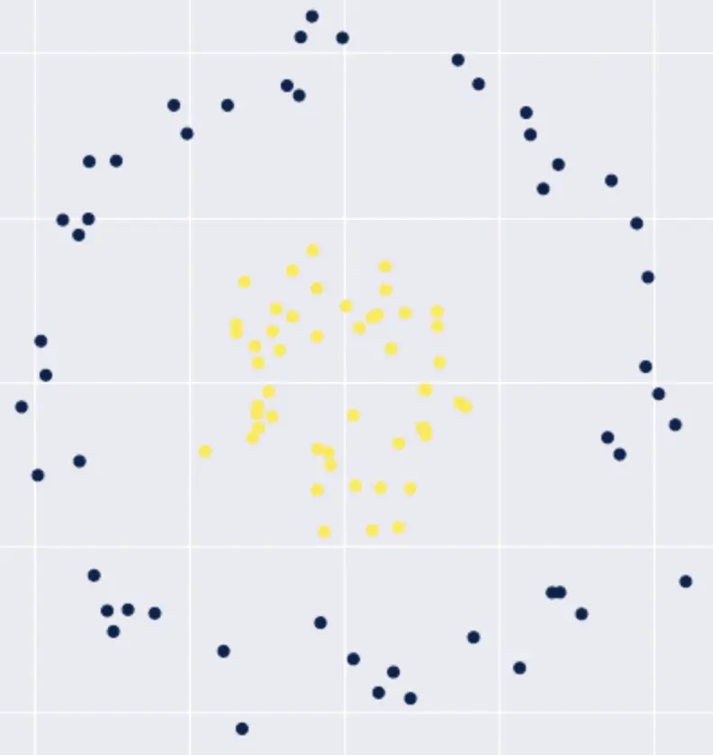
We would have to fit a polynomial function to separate the data, which complicates our classification problem. But what if we could transform this data into a higher-dimensional (3D) space where the data is separable by a linear classifier?
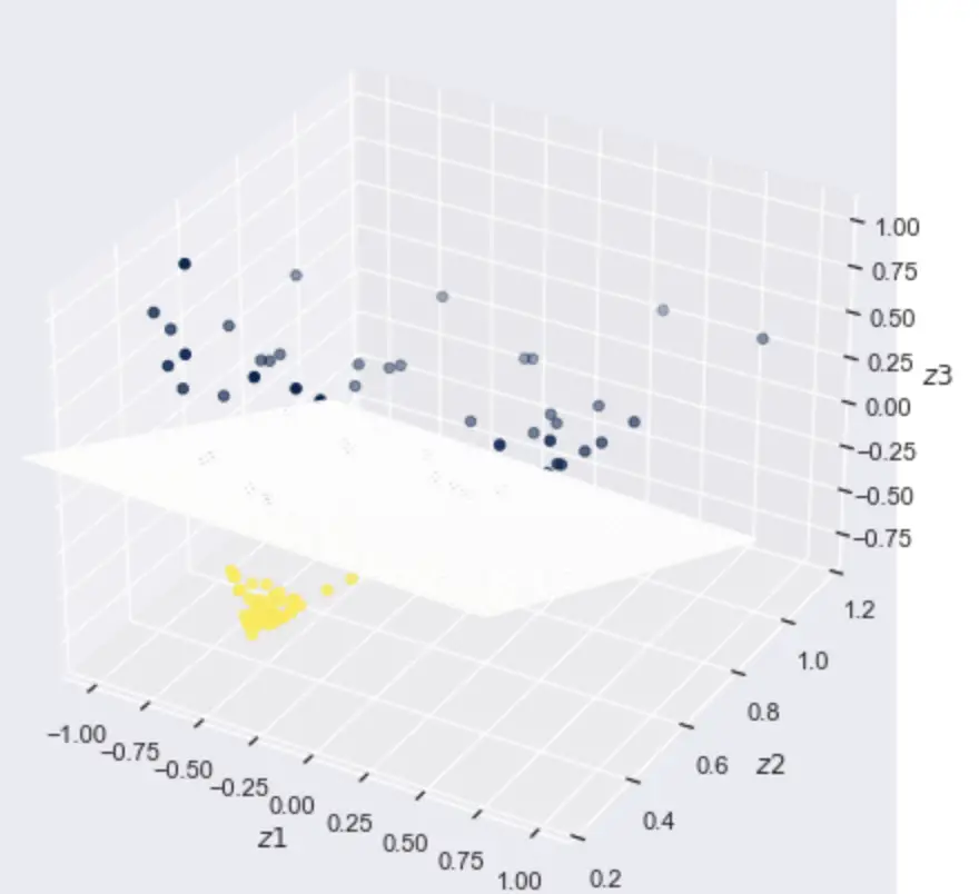
If we can find a mapping from the 2D space into the 3D space where our observations are linearly separable, we can
- Transform our data from 2D into 3D
- Find a linear decision boundary by fitting a linear classifier (a plane separating the data) in the 3D space
- Map the linear decision boundary back into 2D space. The result will be a non-linear decision boundary in 2D
So we’ve essentially found a non-linear decision boundary while only doing the work of finding a linear classifier.
But wait a minute…
To build a linear classifier, we’ve had to transform our data into 3D space. Doesn’t this make the whole operation significantly more complicated?
It turns out with Kernels and the Kernel trick; we can have our cake and eat it too by finding a linear decision boundary in a 3D space while working only with data in the 2D space.
Let’s see how exactly we can achieve this.
What is a Kernel?
We’ve established that a Kernel helps us separate data with a non-linear decision boundary using a linear classifier. To understand how this works, let’s briefly recall how a linear classifier works.
Role of the Dot Product in Linear Classifiers
Consider a linear regression model of the following form:
y_i = w_0 + w_1x_i +w_2x_i + \epsilon_1
If we package all weights into a vector w = {w_0, w_1, w_2} we can express this as a simple dot product between the weight vector and the observation x_i.
y_i = w^Tx_i + \epsilon_1
The dot product between x_I and the weights gives us the predicted point on the line for the actual observation y_i. The difference is the error ε_1
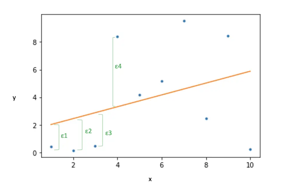
In other words, the dot product is central to the prediction operation in a linear classifier.
Role of the Kernel
Let’s assume we have two vectors, x and x*, in a 2D space, and we want to perform a dot product between them to find a linear classifier. But unfortunately, the data is not linearly separable in our current 2D vector space.
To solve this problem, we can map the two vectors to a 3D space.
x \rightarrow \phi(x) \\
x* \rightarrow \phi(x*)
Where φ(x) and φ(x*) are 3D representations of x and x*.

Now we can perform the dot product between φ(x) and φ(x*) to find our linear classifier in 3D space and then map back to the 2D space.
x^Tx* \rightarrow \phi(x)^T \phi(x*)
But explicitly mapping our features into higher dimensional space is expensive. What if we could find a function that represents the higher-dimensional mapping without actually performing this mapping? This is exactly what a Kernel does.
A Kernel is nothing but a function of our lower-dimensional vectors x, and x* that represents a dot product of φ(x) and φ(x*) in higher-dimensional space.
K(x, x*) = \phi(x)^T \phi(x*)
To illustrate why this works, let’s have a look at a simple Kerne function. All we do is square our dot product.
k(x, x*) = (x^Tx*)^2
Recall that x and x* are vectors in a 2-dimensional input space.
x = [x_1, x_2] \\
x* = [x*_1, x*_2]
If we expand the function, we get the following result.
(x^Tx*)^2 = (x_1 x*_1 + x_2 x*_2) = x_1^2 x*_1^2 + 2 x_1 x*_1 x_2 x*_2 + x_2^2 x*_2^2
This result can be neatly decomposed into the product of 2 3-dimensional vectors.
\phi(x) = \begin{bmatrix}
x_1^2 \\
\sqrt{2}x_1x_2 \\
x_2^2
\end{bmatrix}

\phi(x*) = \begin{bmatrix}
x*_1^2 \\
\sqrt{2}x*_1x*_2 \\
x*_2^2
\end{bmatrix}
The neat thing about Kernels is that we never have to create the full feature map. Instead, we just plug the original Kernel function into our calculation in place of the dot product between x and x*.
k(x, x*) = (x^Tx*)^2
This is a very useful technique that is at the heart of support vector machines. To learn about support vectors and how they work refer to my posts on support vectors and the hinge loss (links open in new tabs).
The Gaussian Kernel
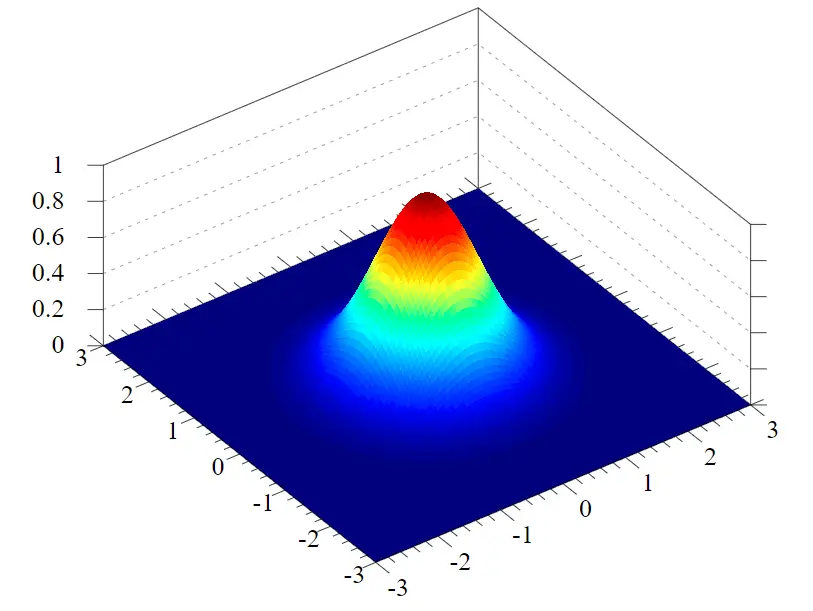
If you are familiar with the Gaussian distribution, you know that it looks like this.
If you are unfamiliar with the Gaussian distribution, here I explain how it works.
Based on the Gaussian distribution, we can construct a kernel that is called the Gaussian kernel. It has the following formula.
k(x, x*) = exp(-\frac{||x-x*||^2}{2\sigma^2})If you take the function apart, you’ll see that part of the function is a measure of the squared distance between x and x*
||x-x*||^2
The other parts of the formula create the specific Gaussian form. Practically speaking, we measure the similarity between the two vectors using the Euclidean distance wrapped into a Gaussian context.
For example, our vectors x and x* would approximately look like this on our Gaussian kernel.
x* = \begin{bmatrix}
0 \\
0
\end{bmatrix}

x = \begin{bmatrix}
-1 \\
-1
\end{bmatrix}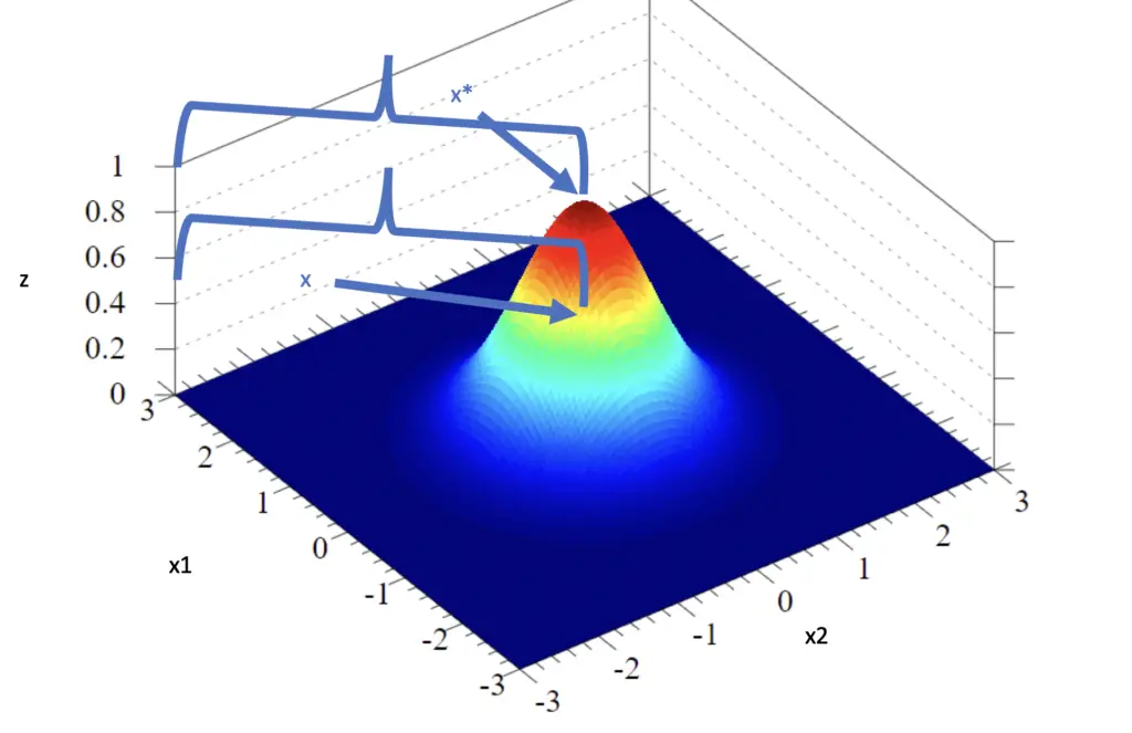
The z-axis measures the output of the Kernel function. The vector x* sits at (0,0), the center of the Gaussian distribution, which has the highest possible similarity of 1 (a vector is completely similar to itself). The vector x sits at the location (-1, -1).
Using the Kernel function, we would like to find its output for the distance between x* and x, which should be a value between 0 and 1. The closer the value to 1, the more similar x is to x*, with 1 indicating that they are identical. From eyeballing the plot, it looks like the z value for the similarity between x* and x should be around 0.5.
First, we have to calculate the Euclidian distance between the two vectors.
||x-x*||^2 = \sqrt{(-1-0)^2 + (-1-0)^2} = \sqrt{2}Then we plug this result into the Gaussian kernel, assuming that the standard deviation σ equals 1.
k(x, x*) = exp(-\frac{\sqrt{2}}{2 \times1^2}) = 0.49The similarity is pretty close to 0.5
When measuring similarity, you can adjust your kernel to become more generous or less generous by adjusting the standard deviation. When you increase the standard deviation, the width of the Gaussian curve increases. Accordingly, values that are further away from the center will have a higher z value. If we set the standard deviation to 2 instead of 1, the kernel function produces a higher similarity for the same vectors and with the same Euclidean distance.
k(x, x*) = exp(-\frac{\sqrt{2}}{2 \times 2^2}) = 0.84Applying a Gaussian Kernel
Assume we have a classification scenario with a non-linear decision boundary such as the following.
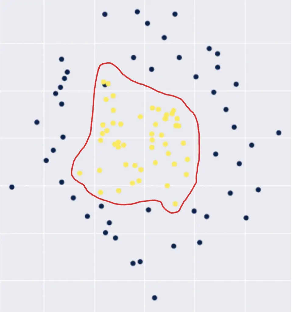
We would have to construct a high-order polynomial to represent this decision boundary in 2-dimensional space.
\theta_0 + \theta_1x_1 + \theta_2x_2 + \theta_3x_2^2 +...
We predict that an observation lies within the decision boundary if the result of our polynomial is greater than 0 and that it lies outside otherwise.
    \hat y=
\begin{cases}
    1 ,& \text{if } \theta_0 + \theta_1x_1 + \theta_2x_2 + \theta_3x_2^2 +...\geq 0\\
    0,              & \text{otherwise}
\end{cases}
We can create a linear classifier using the Gaussian kernel by simply replacing all expressions of x with a Gaussian kernel function.
k_1 = K(x_1, x*)\\
k_2 = K(x_2, x*) \\
k_3 = K(x_2^2,x*)
    \hat y=
\begin{cases}
    1 ,& \text{if } \theta_0 + \theta_1k_1 + \theta_2k_2 + \theta_3xk_3 +...\geq 0\\
    0,              & \text{otherwise}
\end{cases}
But where does x* come from? There are several approaches to constructing the vector x*. For one approach, I suggest watching the following video by Andrew Ng, who does a superb job at explaining it.
Note that Andrew calls the output of the kernel function f instead of k and the second vector l instead of x*. This video is part of his amazing Coursera course. The course has been replaced on Coursera by a brand new machine learning specialization also taught by Andrew. Check it out here.
How to Construct Kernels
We looked at a simple polynomial Kernel where we replaced a dot product in 2-dimensional space with a quadratic kernel function. We determined that this function constitutes a valid mapping to a 3D space by expanding terms and decomposing them into two vectors.
But how can we know whether a function is a valid Kernel without explicitly mapping it to a higher-dimensional space?
The Gram Matrix
Every kernel has an associated Kernel matrix, also known as Gram matrix, where each entry in the matrix equals
G_{ij} = k(x_i, x_j)given the dataset X = {x_1, x_2, …,x_n}. The associated function is a valid Kernel if and only if the Gram matrix is symmetric and positive semi-definite for all possible choices of the dataset X.
The gram matrix is the dot product of the feature representations in the higher-dimensional vector space.
G_{ij} = \phi(x_i)^T\phi(x_j)For linear kernels, it is simply the dot product of the vectors in the original space. If you are interested in how to construct this matrix, I strongly suggest you check out Chapter 6 on Kernel methods in the book “Pattern Recognition and Machine Learning” by Christopher Bishop.
For our purposes, it is enough to know that the Gram matrix allows for the construction of several different types of kernels, such as polynomial kernels, Gaussian kernels, and sigmoid kernels. For deeper coverage on constructing Kernels in practice, I’d like to refer you again to Chapter 6.2. in the book “Pattern Recognition and Machine Learning”.
Summary
Kernels in machine learning can help to construct non-linear decision boundaries using linear classifiers. They achieve this by mapping features to higher-dimensional vector spaces using functions that represent dot products in the higher dimension without explicitly creating those feature mappings.
A Kernel can be considered a similarity function, and there are several types of kernels to calculate that similarity, such as polynomial and Gaussian kernels.
This post is part of a larger series I’ve written on machine learning and deep learning. For a comprehensive introduction to deep learning, check out my blog post series on neural networks. My series on statistical machine learning techniques covers techniques such as linear and logistic regression.

