Stochastic Gradient Descent versus Mini Batch Gradient Descent versus Batch Gradient Descent

In this post, we will discuss the three main variants of gradient descent and their differences. We look at the advantages and disadvantages of each variant and how they are used in practice.

Batch gradient descent uses the whole dataset, known as the batch, to compute the gradient. Utilizing the whole dataset returns a gradient that points directly towards the local or global optimum, resulting in a smooth descent. Due to its computational inefficiency, batch gradient descent is rarely used in practice.

Stochastic gradient descent refers to the practice of performing gradient descent using single samples. Since the samples are randomly selected, the gradients will oscillate, making stochastic gradient less likely to get stuck in local minima than batch gradient descent. Furthermore, we don’t have to wait until the gradient on the entire dataset has been calculated, which makes it much more suitable for practical applications with big datasets.

Mini batch gradient descent is the practice of performing gradient descent on small subsets of the training data. Using several samples will reduce the oscillations inherent in stochastic gradient descent and leader to a smoother learning curve. At the same time, it is more efficient than batch gradient descent in practice since we don’t have to calculate the gradient of the entire dataset at once.

Gradient Descent Recap

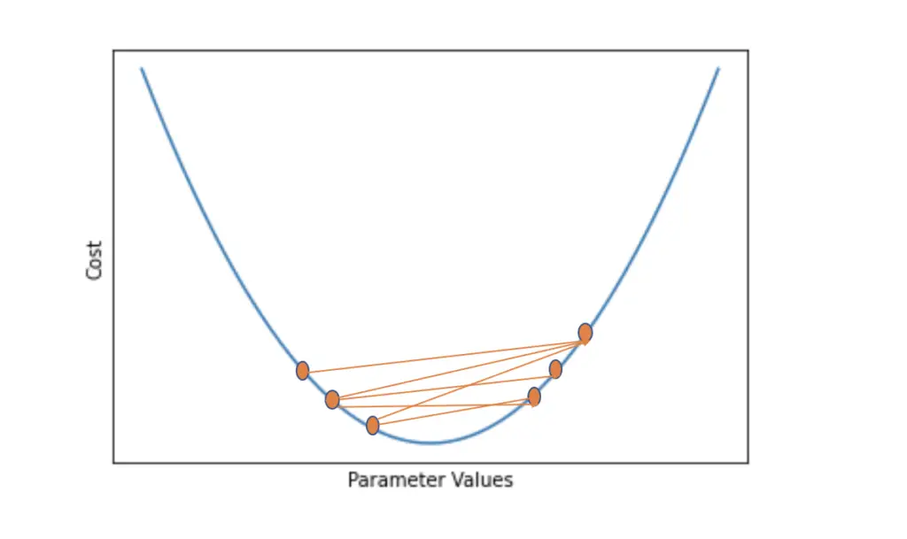
The aim of all variants of gradient descent is to optimize the parameters of a function with the goal of reducing the cost. The algorithm attempts to achieve this by calculating the gradient of the cost function with respect to the parameters. The gradient will point in the direction of the steepest ascent.

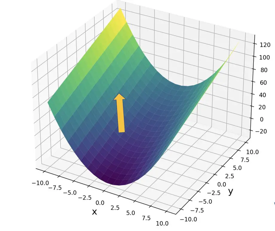
By going in the opposite direction and subtracting the gradient from the current parameter values, we approach the optimal parameter values that minimize the cost function.

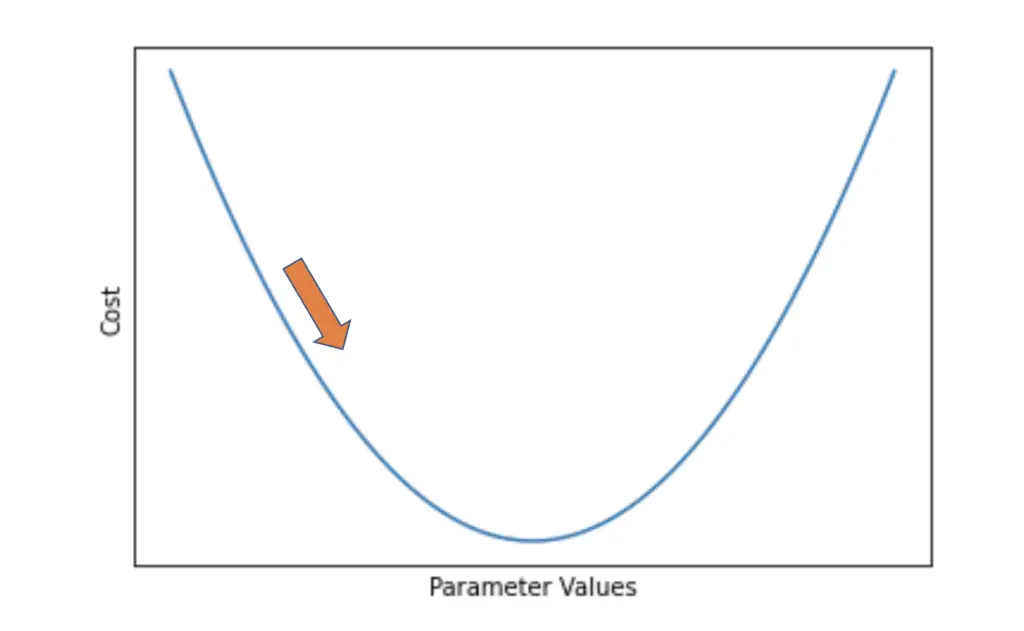
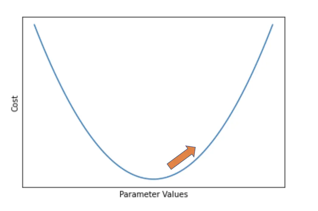
As soon as we move one step in the direction of the steepest descent, the gradient will change. Therefore, we need to iteratively recalculate the gradient after every couple of steps. If we take too many steps in one direction or our step size is too big, we may overshoot the minimum.

If you want a more detailed introduction to gradient descent, check out my posts on the math behind gradient descent and a step-by-step explanation of backpropagation with gradient descent.

Assume we want to learn a function f that takes our input data x and a parameter vector theta as inputs and aims to produce an output y.

f(x, \theta) \; \\y

The inputs x and expected outputs y represent our dataset, and each contains a number I samples.

x = [x_1, x_2, ...,x_I] \\
y = [y_1, y_2, ...,y_I]

We want to optimize the parameters theta using gradient descent. So we define a cost function J that quantifies the difference between the output produced by f and the actual value y.

J(f(x, \theta) ,\;y)

Batch Gradient Descent

In batch gradient descent, we calculate the gradient of the cost function over the entire dataset.

\nabla J(f(x, \theta) ,\;y)

Then we subtract the gradient from our current value of theta multiplied by a step size alpha (we use alpha to scale down the gradient and prevent us from overshooting the minimum).

\theta = \theta - \alpha \nabla J(f(x, \theta) ,\;y)

In practice, batch gradient descent is not a viable option due to two reasons.

Getting Stuck in a Local Minimum

Since we are calculating the gradient of the entire training dataset, gradient descent leads us smoothly to the nearest minimum. If the training problem is convex, meaning that there is only one minimum, this isn’t a problem. But imagine we had a function with multiple minima like the following.

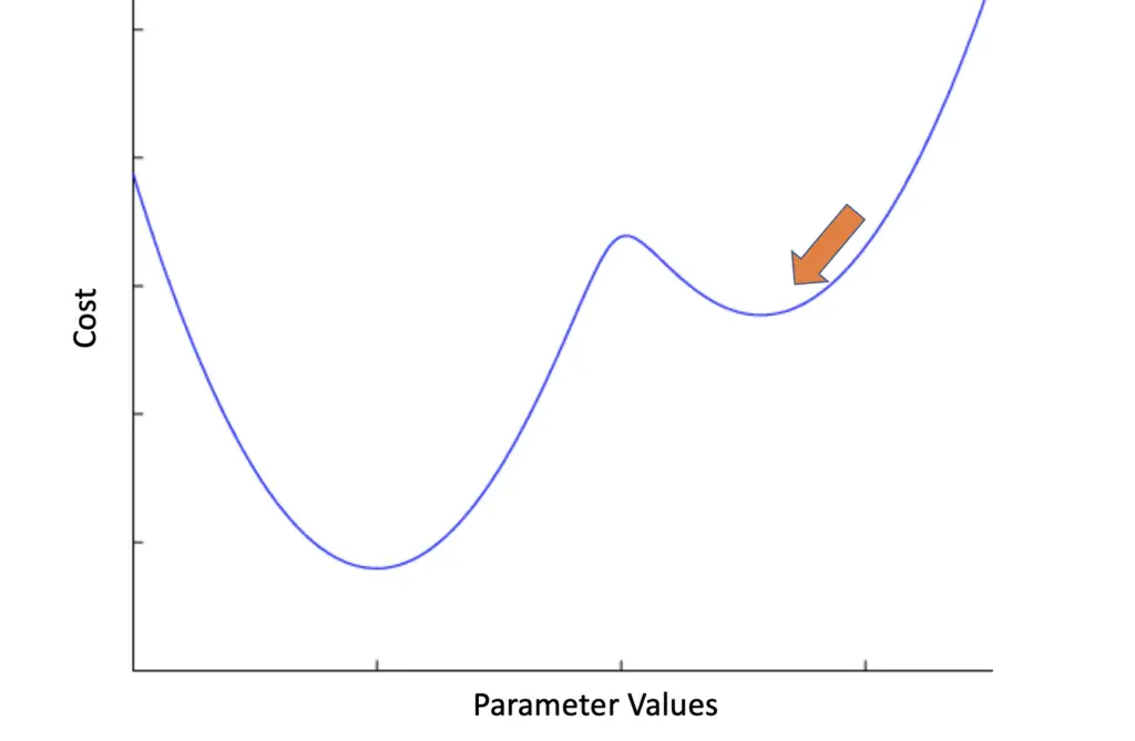
Batch gradient descent might get stuck in the nearest local minimum without finding the global minimum. This is equivalent to getting stuck between two hills in the dark on the way into the valley. To get to the valley, you first have to climb over another hill. The strategy of always going downhill until you reach the valley breaks down at this point.
As we will see, stochastic gradient descent and mini-batch gradient descent are better equipped to get gradient descent out of local minima.

Computational Inefficiency

Now imagine our dataset consisted of 100 000 training examples with 5 features. Calculating the gradient across all of these examples and features requires 500 000 calculations at training every iteration.
Remember that we have to recalculate the gradient after every step we take. When training neural networks, we commonly take several hundred or thousands of steps called training iterations.
Let’s say we use 1000 iterations. In total, we would have to perform 500 million calculations.

5 \times 100\;000 \times 1000 = 500 \;000\;000

This approach would take a very long time to converge. Furthermore, you are likely to run into memory limitations depending on the hardware you are using since the entire dataset has to be loaded into memory and used for computation.

Stochastic Gradient Descent

Stochastic gradient descent calculates gradients on single examples rather than the whole batch. So instead of using the entire data vectors x and y, you pick a random sample consisting of x_i and y_i, calculate the gradient, and perform the update.

\theta = \theta - \alpha \nabla J(f(x_i, \theta) ,\;y_i)

Instead of 500 million calculations, we only have to perform 5000 calculations which is much faster.

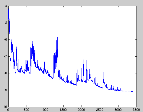
Furthermore, the random choice of a training example introduces randomness into the training process. Since you are not calculating the gradient over the entire dataset, you won’t get a gradient that smoothly leads you straight to the next minimum. Single examples may have different gradients, so the loss might even increase temporarily, and the learning graph showing the loss over several iterations will oscillate much more.

In aggregate, you will still move towards the minimum because the average of the steps you take will point you towards the minimum. Furthermore, the oscillations in the gradient values will help you get out of local minima.
If you were walking down a mountain at night and you had a device that calculated the slope across the entire trail from the peak to the valley, it would always point you straight downwards. If you followed the guidance of the device and you got stuck between two hills, you would be stuck there forever. According to your device, you would have to go straight down rather than first climbing over the next hill. That is the problem with batch gradient descent.
Now imagine your device always calculated the slope based on some random section of the trail. Since some sections of the trail will temporarily lead uphill, the device will sometimes tell you to go uphill. Thus, it will help you get out of the situation where you are stuck between two hills and eventually lead you to the valley.

Thus, stochastic gradient descent effectively addresses the computational inefficiency and tendency to get stuck in local minima that we encountered with batch gradient descent. Because it calculates gradients on single samples, it is also appropriate for online learning in a production system, where you continuously have new data flowing in.

But due to the stochasticity and the resulting fluctuations in the cost, stochastic gradient descent has a harder time converging to the exact minimum. Instead, it is likely to overshoot the minimum repeatedly without properly settling down.

An approach to address this problem is to gradually reduce the learning rate or step size as gradient descent converges on the minimum. That way, the steps become smaller the closer the algorithm gets to the minimum, making it less likely to overshoot.

Mini Batch Gradient Descent

Mini batch gradient descent is a compromise between batch gradient descent and stochastic gradient descent that avoids the computational inefficiency and tendency to get stuck in the local minima of the former while reducing the stochasticity inherent in the latter. Accordingly, it is most commonly used in practical applications.

Rather than performing gradient descent on every single example, we randomly pick a subset of size n of the batch (without replacement) and perform gradient descent.

\theta = \theta - \alpha \nabla J(f(x_{i:i+n}, \theta) ,\;y_{i:i+n})

The size of the minibatch is usually chosen to the power of two, such as 32, 64, 128, 256, 512, etc. The more memory you have available on your hardware, the larger mini-batches you can pick although the ability of the model to generalize might suffer if you pick larger mini-batches.

Since we are using several training examples to calculate the gradient, the stochasticity is reduced, and the algorithm is less likely to overshoot. Still, overshooting can occur if the learning rate is too big, while learning will become slow if it is too small. Choosing an appropriate learning rate remains a challenge with mini-batch gradient descent, which is more art than science and mainly comes down to experience.

This article is part of a blog post series on the foundations of deep learning. For the full series, go to the index.