The Sigmoid Function and Binary Logistic Regression

In this post, we introduce the sigmoid function and understand how it helps us to perform binary logistic regression. We will further discuss the gradient descent for the logistic regression model (logit model).

In linear regression, we are constructing a regression line of the form y = kx + d. Within the specified range, the output y can assume any continuous numeric value along the regression line.

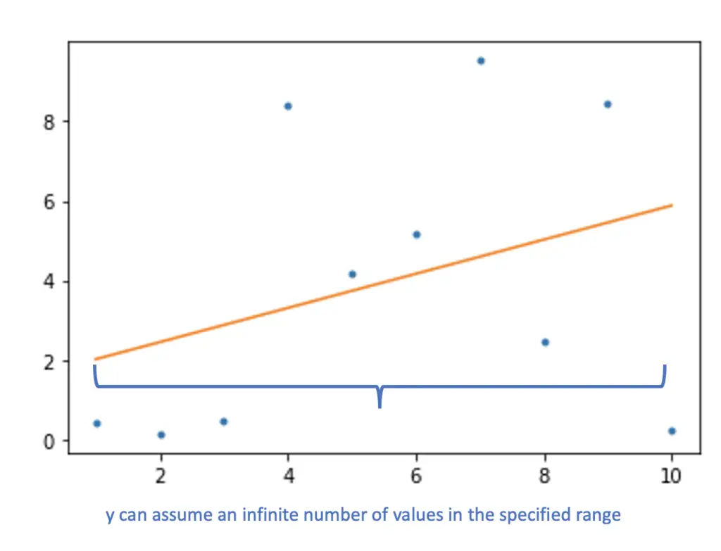
When dealing with a classification problem, we want the model to return one of a limited number of discrete classes. Therefore, a regression model isn’t a suitable solution for classification problems.

In the following video, Andrew Ng does an amazing job demonstrating what happens when you do try to use a regression model in a classification setting. This video is from his Coursera course on machine learning.

What is the Sigmoid Function?

The sigmoid function turns a regression line into a decision boundary for binary classification.

If we take a standard regression problem of the form

z = \beta^tx

and run it through a sigmoid function

\sigma(z) = \sigma(\beta^tx)

we get the following output instead of a straight line.

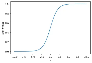
Binary Logistic Regression

As you can see, the sigmoid is a function that only occupies the range from 0 to 1 and it asymptotes both values. This makes it very handy for binary classification with 0 and 1 as potential output values. When a linear regression model gives you a continuous output like -2.5, -5, or 10, the sigmoid function will turn it into a value between 0 and 1.

\left\{
    \begin{array}{l}
      \sigma(z) < 0.5 &\quad if \; z<0 \\
      \sigma(z) \geq 0.5 &\quad if \; z\geq0 \\
    \end{array}
  \right.

You can interpret this as a probability indicating whether you should sort the output into class 1 or class 0. If the value returned by the sigmoid function is below 0.5, you sort it into class 0. Otherwise, you sort it into class 1. So in practice, the logistic regression model makes the following predictions:

\hat y =   
\left\{
    \begin{array}{l}
      0 &\quad if \; \sigma(z) < 0.5 \\
      1 &\quad if \; \sigma(z) \geq 0.5 \\
    \end{array}
  \right.

If you are familiar with hypothesis testing in statistics, you can posit this problem as a hypothesis. The hypothesis beta given input x denotes the probability that the outcome falls into class 1.

h_\beta(x) = \sigma(\beta^tx)

Assume your sigmoid function is tasked with classifying credit card transactions as fraudulent or not. If the function returns a 70% probability that the transaction is fraudulent, you would write:

h_\beta(x) = 0.7

If the linear regression model returns 2.5, 5, or 10 the sigmoid function will sort it into the class associated with 1.

Sigmoid Function Formula

The sigmoid function is a special form of the logistic function and has the following formula.

\sigma(z) = \frac{1}{1+e^{-z}}

Common to all logistic functions is the characteristic S-shape, where growth accelerates until it reaches a climax and declines thereafter.

As we’ve seen in the figure above, the sigmoid function is limited to a range from 0 to 1.

Loss Function For Logistic Regression

In linear regression, we’ve been able to calculate the minimum value for the sum of squared residuals analytically. For logistic regression, this isn’t possible because we are dealing with a convex function rather than a linear one. In practical machine learning applications, we commonly use the gradient descent algorithm to iteratively find the global minimum.

To get gradient descent to find the global minimum, we need to define a loss function (also known as the cost function) for the parameters of our logistic regression model which the gradient descent tries to minimize. The cost function imposes a penalty for classifications that are different from the actual outcomes. For the logistic regression cost function, we use the logarithmic loss of the probability returned by the model.

cost(\beta) =   
\left\{
    \begin{array}{l}
      -log(\sigma(z)) &\quad if \; y=1 \\
       -log(1-\sigma(z)) &\quad if \; y=0 \\
    \end{array}
  \right.

To understand why we use the logarithm here, let’s first have a look at the curve for the two cost functions between 0 and 1 on the x-axis.

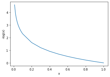
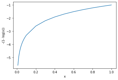
As you can see, -log(x) explodes towards infinity as we approach zero on the x-axis and flattens until it reaches 0 as x approaches 1. Its inverse -(1-log(x)) has exactly the opposite behavior.

Why do we want our loss function for logistic regression to behave this way rather than in a linear fashion?

Imagine your model is employed in a medical setting and it is 100% certain that the cough of a patient is the result of a cold instead of lung cancer. But a few months later it turns out that the patient did have lung cancer. Now, the disease has progressed to a stage where it is incurable.

You don’t want your model to give you certainty in critical scenarios where things can only be determined probabilistically. The closer your model gets to certainty, the more you punish your model with a disproportionately higher cost. You essentially make 100% certainty impossible by letting the cost explode to infinity.

Here is the full cost function with m representing the number of samples :

Cost(\beta) = -\frac{1}{m} \sum^m_{i=1} [y_i \;log(\sigma(z)_i) + (1-y_i)log(1-\sigma(z)_i)]

To see why this function works intuitively, let’s take a single observation and say the actual outcome y is 1 and the probability returned by the model is 0.99. So the model is extremely confident that the outcome is 1.

1 \times log(0.99) + (1-1)\log(1-0.99)= -0.01

Since y equals 1, the second term is zero, and our loss is very small.

Let’s say the actual outcome is zero.

0 \times log(0.99) + (1-0)\log(1-0.99)= -4.6

Now, the situation has been reversed. The first term is zero and our model has been heavily penalized because it was very confident that the outcome y was 1, while it was actually 0.

Logistic Regression with Gradient Descent

The gradient is the vector that points us in the direction of the steepest ascent. To find the minimum, we need to go in the opposite direction of where the gradient is pointing by subtracting our gradient from the initial cost.
We find the gradient by taking the first partial derivative of the cost with respect to each parameter in β. β is a vector of j entries.

Starting from our initial cost function

Cost(\beta) = -\frac{1}{m} \sum^m_{i=1} [y_i \;log(\sigma(\beta^tx_i)) + (1-y_i)log(1-\sigma(\beta^tx_i))]

we take the partial derivative of the cost with respect to every β_j. What we get is the gradient vector of j entries pointing us in the direction of steepest ascent on every dimension j in β. Skipping over a few steps, this is the final outcome:

\frac{\partial Cost(\beta)}{\partial \beta_j} = -\frac{1}{m} \sum^m_{i=1} [\sigma(\beta^tx_i) - y_i)x_{ij}

If you have strong foundations in calculus, I invite you to check this for yourself. Otherwise, forget about it or check out my series on calculus for machine learning.

Since we don’t know how far we have to go and we don’t want to overstep the minimum, we iteratively subtract the gradient multiplied by a small value α from our cost.

Cost(\beta) = Cost(\beta) - \alpha \frac{\partial Cost(\beta)}{\partial \beta_j} 

That’s it. You now know how a binary logistic regression model works. This should give you a good foundation for tackling neural networks and deep learning.

To understand how logistic regression works in settings with more than two classes, check out my post on multinomial logistic regression. I’ve also written a post on how to perform logistic regression in Python.