Logistic Regression in Python

In this post, we are going to perform binary logistic regression and multinomial logistic regression in Python using SKLearn.

If you want to know how the logistic regression algorithm works, check out this post.

Binary Logistic Regression in Python

For this example, we are going to use the breast cancer classification dataset that comes with Scikit Learn. It consists of 30 features that we will use to predict whether a tumor is benign or malignant.

First, we import all the necessary packages. We use NumPy and pandas for representing our data, matplotlib for plotting, and sklearn for building and evaluating the model

import matplotlib.pyplot as plt
import numpy as np
import pandas as pd
from sklearn.linear_model import LogisticRegression
from sklearn.metrics import classification_report, confusion_matrix, plot_confusion_matrix
from sklearn.model_selection import train_test_split
from sklearn import datasets

Next, we import the dataset consisting of 30 predictor variables and one target variable (whether the tumor is malignant or not).

dataset = datasets.load_breast_cancer()
X = dataset.data
y = dataset.target

Now, our dataset X is a NumPy array of 569 x30 dimensions. I generally find it more convenient to work with pandas dataframes as it makes a visual inspection of the data easier. For most models, it doesn’t matter whether you pass data as a NumPy array or a pandas data frame. We use the DataFrame function to construct a data frame. This requires us to pass the raw data along with the name of the features which will become the column names. Let’s also print the first couple of rows to see what it looks like.

X = pd.DataFrame(X, columns = dataset.feature_names)
X.head()

Next, we use SKlearn to split the data into a training set and a testing set. We also tell the function to allocate 75% to the training set and 25% to the test set. This dataset is fairly small, so this seems like a reasonable split. The random state variable allows you to reproduce the same split. In this case, it is irrelevant.

X_train,X_test,y_train,y_test = train_test_split(X,y,test_size=0.25,random_state=0)  

Now, we can create our logistic regression model and fit it to the training data.

model = LogisticRegression(solver='liblinear', random_state=0)
model.fit(X_train, y_train)

Our model has been created. A logistic regression model has the same basic form as a linear regression model. It has an intercept and slope parameters for every feature dimension. Since we have thirty dimensions, there should be 30 slopes. Let’s have a look at these parameters.

print("intercept:")
print(model.intercept_)
print("slopes:")
print(model.coef_)

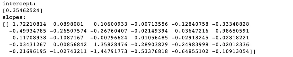
The output is as expected. We get a single intercept and 30 slopes.

Finally, we can make predictions on the test data using our newly trained model.

preds = model.predict(X_test)
print(preds)
'''
array([0, 1, 1, 1, 1, 1, 1, 1, 1, 1, 1, 1, 1, 0, 1, 0, 1, 0, 0, 0, 0, 0,
       1, 1, 0, 1, 1, 0, 1, 0, 1, 0, 1, 0, 1, 0, 1, 0, 1, 0, 0, 1, 0, 1,
       0, 0, 1, 1, 1, 0, 0, 0, 0, 1, 1, 1, 1, 1, 1, 0, 0, 0, 1, 1, 0, 1,
       0, 0, 0, 1, 0, 0, 1, 1, 0, 1, 1, 1, 1, 1, 0, 0, 0, 1, 0, 1, 1, 1,
       0, 0, 1, 0, 0, 0, 1, 1, 0, 1, 1, 1, 1, 1, 1, 1, 0, 1, 0, 1, 0, 0,
       1, 0, 0, 1, 1, 1, 1, 1, 1, 1, 1, 1, 0, 1, 0, 1, 0, 1, 1, 1, 0, 1,
       1, 1, 1, 1, 1, 0, 0, 1, 1, 1, 0])
'''

The predict function returns an array of 1s and 0s depending on whether the tumor has been classified as malignant (1) or benign (0).

A breast cancer diagnosis is a life-altering event. As someone who builds these types of models you have an ethical responsibility to ensure that the model works well.

So let’s check how the model performs on unseen data. SciKit-Learn makes this very easy with the score function which you can simply call on your trained model. We just need to pass the test data.

model.score(X_test, y_test)
# 0.9580

Our model has an accuracy of 95%. But accuracy is often not enough. With breast cancer diagnoses a false positive is less problematic than a false negative. In the first case, the woman might get an initial shock which will hopefully be relieved after a follow-up test. In the second case, the woman goes home glad that she is healthy, while she actually has cancer. So we want to avoid false negatives even at the cost of increasing false positives.

We can see how many false positives and false negatives as well as true positives and true negatives our model has produced by creating a confusion matrix.

A confusion matrix plots the predicted values vs the true label.

plot_confusion_matrix(model, X_test, y_test)
#

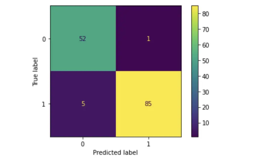
As you can see, the test has 5 false negatives (True 1, Predicted 0) and 1 false positive (True 0, Predicted 1). Out of 143 women who came for a breast cancer check, we’ve sent 5 women home telling them they are fine while they actually have cancer. In a real-life scenario, this would not be a satisfying performance! But for the sake of demonstration we are going to leave it like this.

Multinomial Logistic Regression in Python

For multinomial logistic regression we are going to use the Iris dataset also from SKlearn. This dataset has three types fo flowers that you need to distinguish based on 4 features.

The procedure for data loading and model fitting is exactly the same as before. SKlearn is smart enough to adjust the model based on the target variable. So I’ll just give you the full code.

dataset = datasets.load_iris()
X = dataset.data
y = dataset.target

#we skip converting X to a dataframe

X_train,X_test,y_train,y_test = train_test_split(X,y,test_size=0.25,random_state=0)  #in this case, you may choose to set the test_size=0. You should get the same prediction here

model = LogisticRegression(solver='liblinear',  random_state=0)
model.fit(X_train, y_train)

When we perform a prediction on the test data, we get 3 classes (0,1,2).

preds = model.predict(X_test)
print(preds)

The confusion matrix now is 3×3 rather than 2×2

plot_confusion_matrix(model, X_test, y_test)

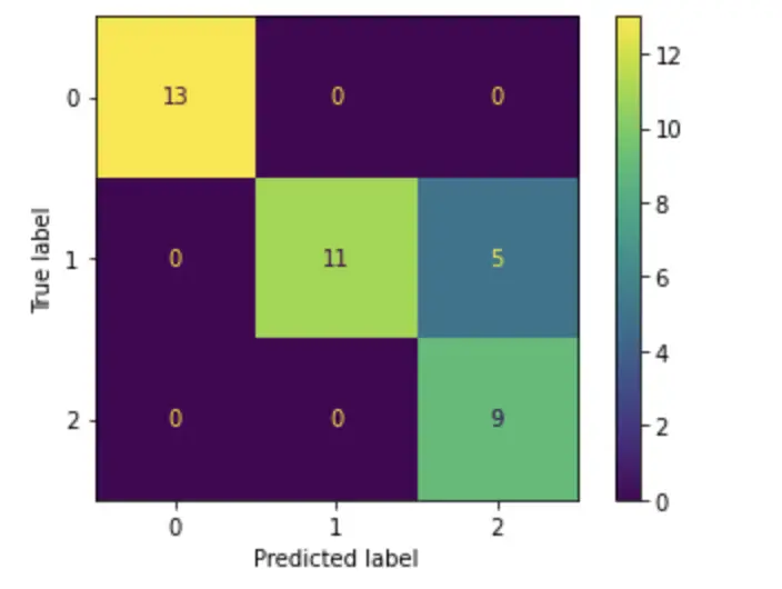
The correctly classified instances are listed along the main diagonal. It seems the model is doing a superb job with one exception: It classified several instances that belong to category 1 into category 2.

You now know how to perform logistic regression in Python.