The Softmax Function and Multinomial Logistic Regression

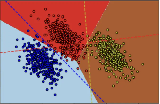
In this post, we will introduce the softmax function and discuss how it can help us in a logistic regression analysis setting with more than two classes. This is known as multinomial logistic regression and should not be confused with multiple logistic regression which describes a scenario with multiple predictors.

What is the Softmax Function?

In the sigmoid function, you have a probability threshold of 0.5. Those observations with a probability below that threshold go into class A. Those with a probability above the threshold go into class B. Accordingly, you are limited to a prediction between two classes.

In multiple logistic regression we want to classify based on more than two classes.

To be able to classic between more than two classes, you need a function that returns a probability value for every class. The sum of all probabilities needs to sum to one. The softmax function suits these requirements.

Softmax Function Formula

softmax(z) = \frac{e^{z(i)}}{\sum^k_{j=0} e^{z(j)}}

where z is a vector of inputs with length equivalent to the number of classes k.

Let’s do an example with the softmax function by plugging in a vector of numbers to get a better intuition for how it works.

z = [1,3,4,7]

If we want to calculate the probability for the second entry, which is 3, we plug our desired values into the formula

softmax(z_2) = \frac{e^3}{e^1+e^3+e^4+e^7} = 0.017

Applying the softmax function to all values in z gives us the following vector which sums to 1:

softmax(z) = [0.002, 0.017, 0.047, 0.934]

As you see, the last entry has an associated probability of more than 90%. In a classification setting, you would assign your observation to the last class.

Multinomial Logistic Regression

You perform multinomial logistic regression by creating a regression model of the form

z = \beta^tx

and applying the softmax function to it:

\hat y = softmax( \beta^tx)

Multinomial Logistic Regression Loss Function

The loss function in a multiple logistic regression model takes the general form

Cost(\beta) = -\sum_{i=j}^k y_j log(\hat y_j)

with y being the vector of actual outputs. Since we are dealing with a classification problem, y is a so called one-hot vector. This means all positions in the vector are 0. Only the entry representing the class that the observations falls into is 1.

Let’s illustrate this with an example:

Suppose you want to classify fruits into one of three categories and the actual fruit is a banana. For the sake of simplicity, we will only look at one observation. The vector y would look like this:

y = 
\begin{bmatrix}
0\\
1\\
0
\end{bmatrix}
=
\begin{bmatrix}
apple\\
banana\\
orange
\end{bmatrix}

You have some data that you train your logistic regression model on and it returns the following prediction vector of probabilities.

\hat y = 
\begin{bmatrix}
0.2\\
0.7\\
0.1
\end{bmatrix}

Now, we plug this into our cost function:

Cost(\beta) = -(0 \times log(0.2) + 1 \times log(0.7) + 0 \times log(0.1)) 

A very convenient feature of this function is that due to their entries in y being 0 all terms that do not relate to the actual true class will disappear:

Cost(\beta) = -log(0.7) = 0.36

This function effectively serves the purpose of minimizing the cost. The larger the probability y_hat associated with the true probability, the smaller the cost.

To find the gradient we take the first derivative of the cost with respect to every entry β_j in β. The derivative is quite simple. It turns out to be

\frac{\partial Cost(\beta)}{\partial \beta_j} = \hat y - y

Finally, we can apply gradient descent to iteratively minimize the cost multiplied by a learning rate α.

Cost(\beta) = Cost(\beta) - \alpha \frac{\partial Cost(\beta)}{\partial \beta_j} 

That’s it, we now know how to perform multiclass classification with logistic regression. Next, we’ll look at an implementation of logistic regression in Python.