Understanding The Gradient Descent Algorithm

In this post, we introduce the intuition as well as the math behind gradient descent, one of the foundational algorithms in modern artificial intelligence.

Motivation for Gradient Descent

In many engineering applications, you want to find the optimum of a complex system. For example, in a production system, you want to find the ideal combination of inputs to maximize the output. Many real-life applications have thousands of inputs. Finding an analytical solution can become prohibitively expensive in terms of computing resources. Many optimization methods, therefore, rely on iterative rather than analytical solutions. Linearization with Taylor polynomials forms the basis of many iterative solutions.

Gradient descent is an iterative optimization method that relies on linear approximations, that is, first-order Taylor polynomials, to the desired function.

How Does Gradient Descent Work?

Let’s take the following function.

f(x,y) = x^2 + 3y

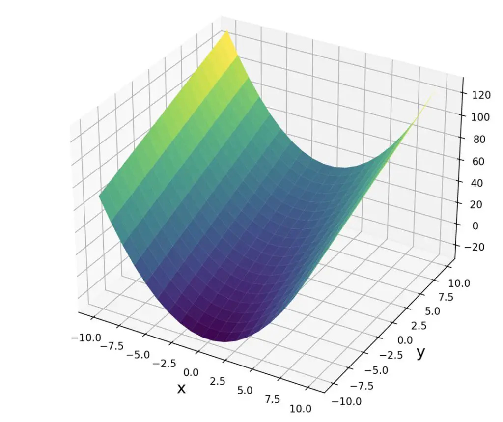
We calculate the gradient across the x and y dimensions by taking the partial derivatives with respect to x and y. The partial derivatives are represented in a Jacobian column vector.

Δf = 
\begin{bmatrix}
    \frac{\partial{f(x,y)}}{\partial{x}} \\
     \frac{\partial{f(x,y)}}{\partial{y}}
  \end{bmatrix}
=
\begin{bmatrix}
    2x \\
     3
  \end{bmatrix}

The gradient vector points you in the direction of the steepest ascent. In non-linear higher-order functions, the direction and steepness will differ depending on where you stand. The gradient of our function f(x,y) is itself a function of x. It, therefore, depends on the location of the evaluation. Accordingly, just following the initial gradient won’t get you anywhere. Instead, you need to take a small step and then reevaluate your new gradient.

Since we want to descend rather than ascend, we need to follow the gradient in the opposite direction. Accordingly, we evaluate our gradient vector at the current position \theta and deduct the gradient vector from the vector indicating our current position.

\theta_1 = \theta_0 - Δf(\theta)

In most practical applications of gradient descent, such as neural network training, deducting the full gradient will be a step that is way too big. We are very likely to overshoot the true minimum. Therefore, deep learning practitioners multiply the gradient with a small number \alpha known as the step size.

\theta_1 = \theta_0 - \alphaΔf(\theta)

Let’s start from a point x0 and apply gradient descent.

x_0 = \begin{bmatrix}
    -10 \\
     10
  \end{bmatrix}

Plugging these values into our Jacobian gradient matrix gives us the following.

Δf = 

\begin{bmatrix}
    2x \\
     3
  \end{bmatrix}
= 
\begin{bmatrix}
    -20 \\
     3
  \end{bmatrix}

Using a step size of 0.1, we can now calculate the next point x1.

x_1 = 


\begin{bmatrix}
    -10 \\
     10
  \end{bmatrix}
-0.1
\begin{bmatrix}
    -20 \\
     3
  \end{bmatrix}
=
\begin{bmatrix}
    -8 \\
     9.7
  \end{bmatrix}

Now we have to calculate the gradient a x1.

Δf = 

\begin{bmatrix}
    2x \\
     3
  \end{bmatrix}
= 
\begin{bmatrix}
    -16 \\
     3
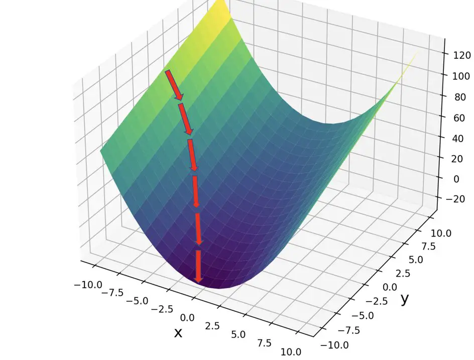
  \end{bmatrix}

This process is repeated many times until we reach the minimum point.

Notice that, as we approach the minimum and the gradient flattens, your step size automatically decreases because x becomes smaller. 0.1 is probably still too large a step size, but you get the idea.

Summary

We’ve learned how to perform gradient descent, one of the foundational algorithms in modern artificial intelligence.

Congratulations! Gradient descent is one of the most difficult concepts in deep learning, especially because it requires solid calculus and linear algebra skills.

This post is part of a series on Calculus for Machine Learning. To read the other posts, go to the index.