Linearization of Differential Equations for Approximation

In this post we learn how to build linear approximations to non-linear functions and how to measure the error between our approximation and the desired function.

Given a well-behaved higher-order function, we can find an approximation using Taylor series. But how do we know when our approximation is good enough so that we can stop adding higher-order terms?

Linearization enables us to measure the error between the linear approximation and the actual function.

Single Variable Taylor Linearization

We start with a linear Taylor polynomial as our approximation function h1(x) to the unknown function f(x) at the point p. This gives us the following form.

h_1(x) = f(p) + f'(p)(x-p)

The expression x-p gives us a distance along the function f(x) that we denote as Δx. Why do we use Δx for error estimation? If we approximate f(x) only at a specific point p, then any function (even the constant p) will be a perfectly accurate approximation. So we can only get an estimate of how good our approximation is if we follow f(x) along a certain distance Δx.

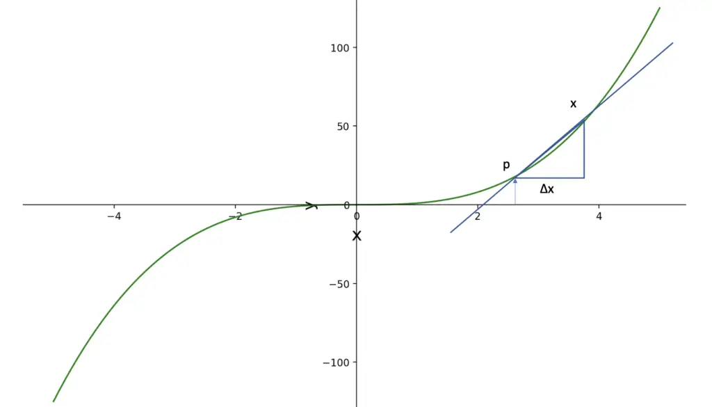
Accordingly, we can replace p-x with Δx. Since we are dealing with a linear approximation, the slope will be the same at every point along h1(x). We can replace the specific point p with the more generic x.

h_1(x) = f(x) + f'(x)Δx

To approximate the real f(x), we can gradually add higher order Taylor terms to h.

h_2(x) = f(x) + f'(x)Δx + \frac{1}{2}f''(x)Δx^2

But now our approximation is not linear anymore. However, we know that Δx must be a relatively small number far below 1. If we square or cube Δx, it will be even smaller. It might be so small, that we can ignore it altogether. The good news is: We can control how small Δx, Δx^2, and all subsequent terms of Δx are.

The point of linearization is to pick a Δx small enough so that we can ignore higher-order terms such as Δx^2, Δx^3.

Rather than using the helper function h(x), we can express the approximation in terms of the unknown function f in terms of x and Δx.

f(x + Δx) = f(x) + f'(x)Δx \color{red} + \frac{1}{2}f''(x)Δx^2 + \frac{1}{6}f'''(x)Δx^3 + ...

f(x+Δx) now constitutes the linear approximation to f(x) within the acceptable error range Δx.

The closer Δx is to zero, the more accurate your approximation, but the smaller the acceptable range in which your approximation is good enough.
You can now express a non-linear function as a series of steps of linear approximations, all of which are acceptably accurate within their respective ranges of Δx. The smaller your Δx, the more steps you need in your approximation.

Linearization is used in many engineering applications ranging from hydraulics to machine learning. What Δx is appropriate, depends on your individual use case.

In machine learning, the idea is fundamental to gradient descent, which is used by neural networks to gradually learn an unknown function.

Multivariable Taylor Series

So far we’ve discussed how to approximate functions with one variable. Real-life applications often have several input variables.

Lets say we wanted to approximate a function f(x,y) across two variables x, and y. To obtain the gradient, we need to take the partial derivatives of f(x,y) with respect to x and y.

f'(x,y) = \partial_x f(x,y)Δx + \partial_y f(x,y)Δy

We’ve discussed how to construct gradients across multiple dimensions and vector-valued functions using the Jacobian matrix, which captures all partial derivatives of a function. Accordingly, we can express the partial derivatives of f(x,y) as a Jacobian matrix.

J_f = [\partial_x f(x,y), \partial_y f(x,y)]

The first-order Taylor polynomial can be expressed in vector form.

f'(x,y) = 
J_f \cdot 
\begin{bmatrix}
Δx\\
Δy
\end{bmatrix}

Thus, we’ve obtained our multivariable linear approximation.

Similarly to obtaining the Jacobian, the second order term in our multivariable approximation

\frac{1}{2}f''(x)Δx^2

can be expressed as a Hessian (remember that the Hessian collects second order derivatives).

\frac{1}{2}Δx^tH_fΔx

Since Δx is now a matrix, we need to multiply by its transpose to obtain higher-order terms.

Δx^2 = Δx\cdotΔx^t

For more in-depth coverage of how we arrive at this expression, check out this excellent video by Khan Academy.

This post is part of a series on Calculus for Machine Learning. To read the other posts, go to the index.