Maximum Likelihood Estimation for Gaussian Distributions

In this post, we learn how to derive the maximum likelihood estimates for Gaussian random variables.

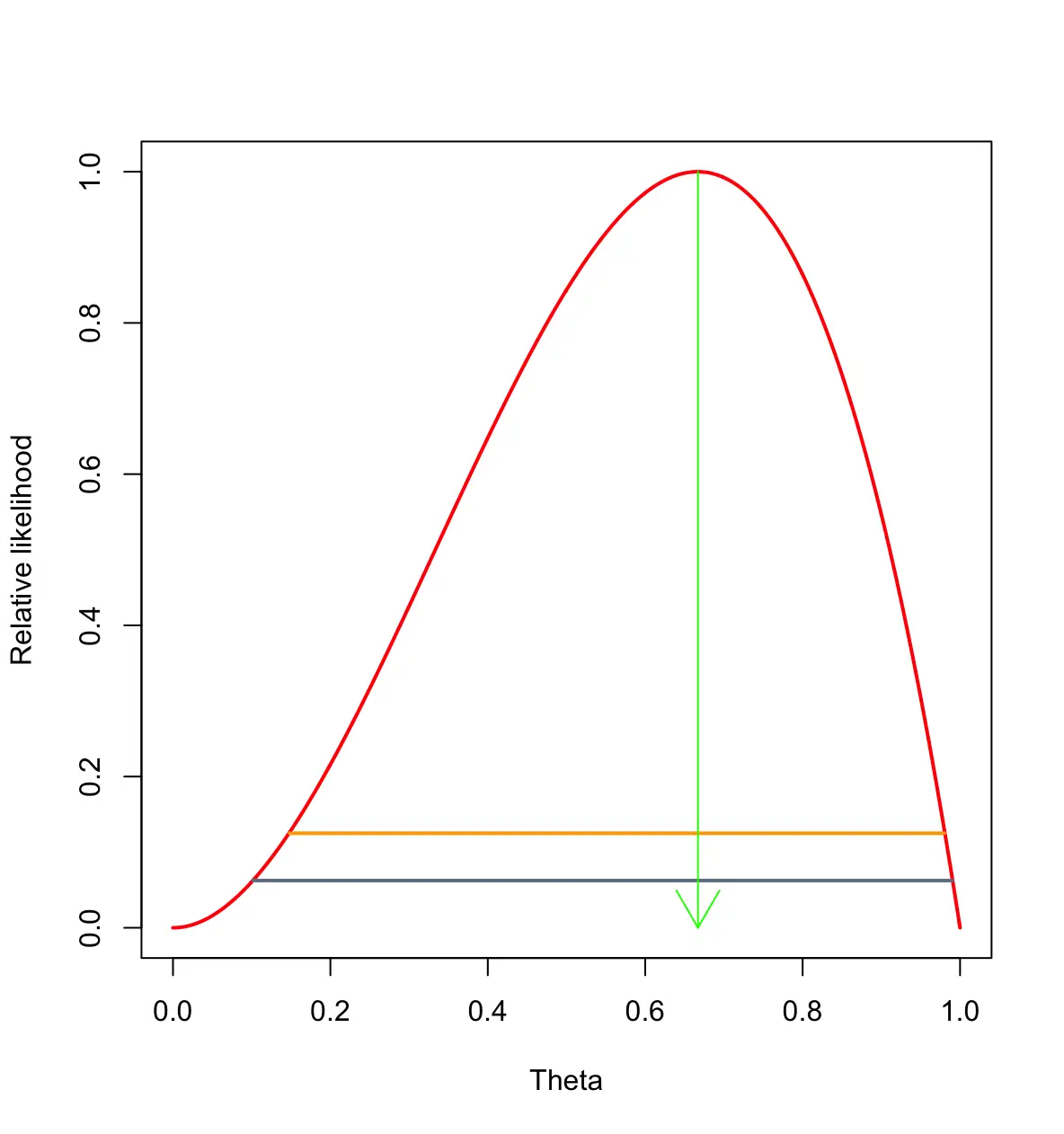
We’ve discussed Maximum Likelihood Estimation as a method for finding the parameters of a distribution in the context of a Bernoulli trial,

Most commonly, data follows a Gaussian distribution, which is why I’m dedicating a post to likelihood estimation for Gaussian parameters.

Gaussian Parameters

A Gaussian distribution has two parameters: mean μ and variance σ. Accordingly, we can define the likelihood function of a Gaussian random variable X and its parameters θ in terms of mean μ and variance σ.

L(X|\theta) = L(X|\mu, \sigma)

This sound fairly abstract, so let’s make this a bit more concrete using an example.

Suppose we wanted to find the parameters that describe the distribution of heights in a certain country. We know that heights follow a normal distribution, but we don’t know the exact mean and variance. We go out and measure the height of 1000 randomly chosen people. The random variable X describes the distribution of heights that we’ve observed.

X = [x_1, x_2, ...,x_{n}]

Based on the data collected we estimate the mean μ and variance σ that are most likely to describe the real distribution of heights given our sample.

In the Bernoulli trials that define a coin flip, we had a set of clearly defined outcomes or realized values. A coin flip can only result in heads or tails. We then tried to find the parameters that are most likely given the outcomes of our trials. When dealing with Gaussian processes, the probability of observing a concrete realized outcome is zero.

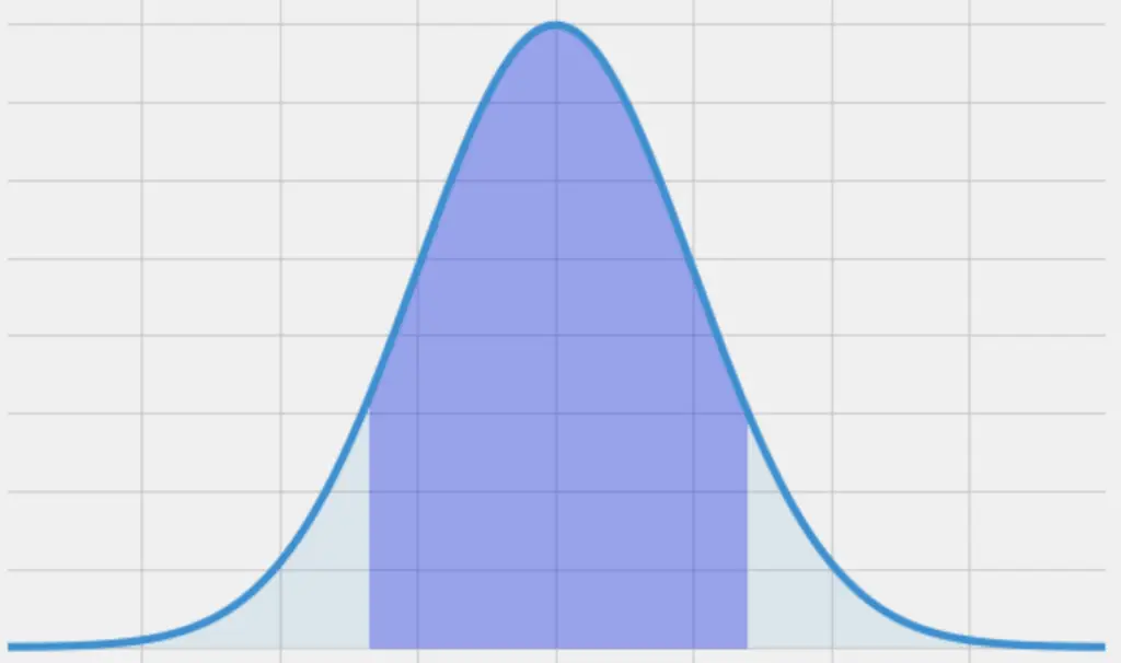
In our example, the probability that we find a person in our sample, who is exactly 6ft (183cm) and not one nanometer taller or shorter, is essentially zero. Instead, we have to think in terms of probability densities or certain areas under the Gaussian curve. For example, we have to ask how probable is it that we observe a height between 5ft and 6ft?

Likelihood as Conditional Probability

We can view the likelihood function as a conditional probability density function of X given θ.

L(X|\theta) = f(X|\theta) = f(X|\mu, \sigma)

We would like to find values for the mean and variance that maximizes the likelihood of obtaining the observed values of X. Given the distribution of heights in our sample, we want to find the parameters μ and σ that are most likely to have generated that data.

\mu _{MLE} = argmax_{\mu} f(X|\mu, \sigma) \\
\sigma_{MLE} = argmax_{\sigma}  f(X|\mu, \sigma) \\

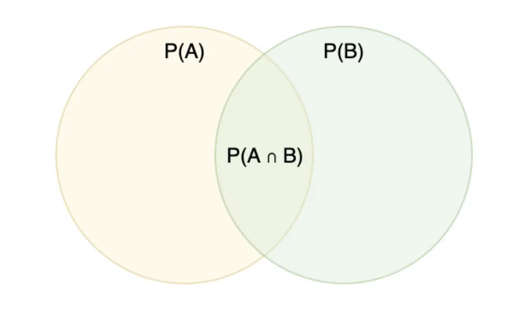
In terms of conditional probability, our observations of heights X are events that have occurred simultaneously.

So we have to find the μ and σ that maximizes the joint probability that all events in X occur.

f(X|\mu, \sigma) = \prod_{i=1}^nf(x_i| \mu, \sigma)

Now the maximum likelihood estimation can be treated as an optimization problem. To find the maximum value, we take the partial derivative of our expression with respect to the parameters and set it equal to zero.

However, there is a neat trick that allows us to reduce the complexity of the calculation. Instead of maximizing the likelihood, we maximize the log-likelihood. The log-likelihood has the advantage of being a monotonically increasing function and it reduces our multiplicative terms to sums. Since the maxima of the likelihood and the log-likelihood are equivalent, we can simply switch to using the log-likelihood and setting it equal to zero.

l = \sum_i^n \nabla_{\mu, \sigma} log(f(x_i| \mu, \sigma)) = 0

Note: the triangle denotes the gradient vector, which expresses the partial derivatives with respect to μ and σ. If this is unfamiliar to you, check out my post on vector calculus.

Deriving the Maximum Likelihood Estimates

Now we can substitute the actual formula for the normal distribution. We are using the natural logarithm of e, so we’ll write ln instead of the log to make it more explicit. Let’s simplify a bit before evaluating the partial derivatives.

l = \sum_i^n \ ln(\frac{1}{\sqrt{2\pi\sigma^2}}e^{(-\frac{(x_i- \mu)^2}{2\sigma^2})}) 

Evaluating the natural log using the quotient and power rules, we get to the following expression:

l = \sum_i^n -\frac{1 }{2}ln(2\pi \sigma^2) {-\frac{(x_i- \mu)^2}{2\sigma^2}} 

The first term that do not depends on i is constant for each value of i. So we can take it out, put it in front of the summation sign and multiply by n. We can also take the divisor of the second term out.

l = -\frac{n }{2} ln(2\pi \sigma^2) 
-\frac{1}{{2\sigma^2}} \sum_i^n  {(x_i- \mu)^2} 

Now, it’s time to evaluate the partial derivatives with respect to μ and σ. Starting with μ, we take the partial derivative of the log-likelihood with respect to μ and set it equal to zero.

\frac{\partial l}{\partial \mu} = \frac{\partial}{\partial \mu} (-\frac{n }{2} ln(2\pi \sigma^2) 
-\frac{1}{{2\sigma^2}} \sum_i^n  {(x_i- \mu)^2}) 

Since we are evaluating the derivative with respect to μ, terms that do not contain μ are constant and disappear when differentiating.

\frac{\partial l}{\partial \mu} =\frac{\partial}{\partial \mu} (
-\frac{1}{{2\sigma^2}} \sum_i^n  {(x_i- \mu)^2}) 

With some more mathematical manipulation, we can show that this is equivalent to.

\frac{\partial l}{\partial \mu} =-\frac{1}{{2\sigma^2}} \sum_i^n \frac{\partial}{\partial \mu} {(x_i- \mu)^2} 

I’ve glossed over some intermediate steps here. If you are interested in the details, check out this post.

Finally we can evaluate the derivative by applying the chain rule

\frac{\partial l}{\partial \mu} =-\frac{1}{{2\sigma^2}} \sum_i^n \frac{\partial}{\partial \mu} {(x_i- \mu)^2} 

\frac{\partial l}{\partial \mu} =-\frac{1}{{2\sigma^2}} \sum_i^n  {2(x_i- \mu) \times-1} 

\frac{\partial l}{\partial \mu} =\frac{1}{{\sigma^2}} \sum_i^n  {(x_i- \mu) } 

Now, it is time to set this expression to zero to find the value for μ that maximizes the log likelihood.

\frac{1}{{\sigma^2}} \sum_i^n  {(x_i- \mu) }  = 0

We divide both sides by σ^2. We can also take μ out of the summation and multiply by n since it doesn’t depend on i.

-n  \mu + \sum_i^n  {x_i }  = 0

Finally we bring μ to the other side by subtracting it and divide the expression by N.

\mu = \frac{1}{n}\sum_i^n  {x_i }

So to obtain our ideal μ, we just have to sum up all the heights we collected in our sample and the divide by the sample size.

But wait, isn’t this the definition of the mean?

Yes, it is. In other words:

The maximum likelihood estimate for the population mean is equivalent to the sample mean.

For the variance, we can apply some similar transformations to our expression for the log-likelihood.

\frac{\partial l}{\partial \sigma} = \frac{\partial}{\partial \sigma} ( -\frac{n }{2} ln(2\pi \sigma^2) 
-\frac{1}{{2\sigma^2}} \sum_i^n  {(x_i- \mu)^2} )

Again, I’ll gloss over several intermediate steps and just present you with the evaluated derivative which we also set equal to zero.

\frac{\partial l}{\partial \sigma} =  -\frac{n }{\sigma} +
\frac{1}{{\sigma^3}} \sum_i^n  {(x_i- \mu)^2} = 0

Bringing the first term to the other side and multiplying by σ^3 gives us the following expression.

n\sigma^2 = 
\sum_i^n  {(x_i- \mu)^2}

Lastly, we divide by n. Remember, that σ is the standard deviation, so σ^2 is the variance.

\sigma^2 = \frac{1}{n}
\sum_i^n  {(x_i- \mu)^2}

This is exactly the formula we use for estimating the variance. Accordingly, the maximum likelihood estimate for the population variance is equivalent to the sample variance.

Summary

We learned to perform maximum likelihood estimation for Gaussian random variables. In the process, we discovered that the maximum likelihood estimate of Gaussian parameters is equivalent to the observed parameters of the distribution of our sample.

This post is part of a series on statistics for machine learning and data science. To read other posts in this series, go to the index.