Power Series: Understand the Taylor and MacLaurin Series

In this post, we introduce power series as a method to approximate unknown functions. We derive the Maclaurin series and the Taylor series in simple and intuitive terms.

Differential calculus is an amazing tool to describe changes in complex systems with multiple inputs. But to unleash the power of Calculus, we need to describe the system in terms of a mathematical function. But how do we find this function in the first place? Power series such as the Taylor series and the MacLaurin series allow us to gradually approximate functions.

The basic idea underlying power series is as follows. If you know a point p along the unknown function f(x) that you are trying to approximate, you can build a function p(x) of increasing orders through that point p until you are as close as possible to f(x).

MacLaurin Series

If we want to approximate an unknown function f(x), the simplest approximation would be a straight line through the point for which x = 0. This gives us our zeroth-order approximation function p0(x), which is just a number a. We’ll use p0(x) and subsequent functions f1(x), f2(x), etc. to construct the polynomial p(x), which is the closest possible approximation of f(x).

p_0(x) = a

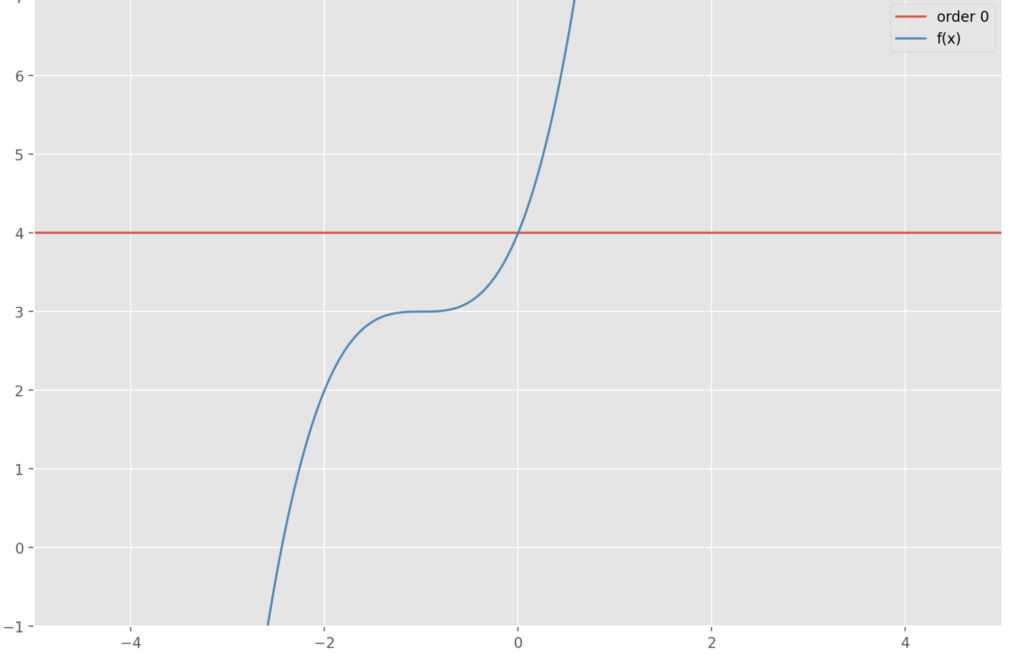
Of course, this isn’t a very useful approximation, but at least we know that our final function p(x) equals f(x) at x = 0. Therefore we can say:

p(0) = f(0)

Instead of just requiring our approximation function to go through the same point at x=0, we add an additional requirement that the slope of p(x) should also be equal to the slope of f(x) at x=0. How do we get to the slope if we don’t know f(x)? Well, we know that the first derivative of a function gives us the slope. So the first derivative of p(x) needs to be equivalent to the first derivative of f(x) at x=0.

p'(0) = f'(0) 

With this knowledge, we can construct a better approximation of p(x) p1(x) of the first order at x = 0.

p_1(x) = f(0) + f'(0)x

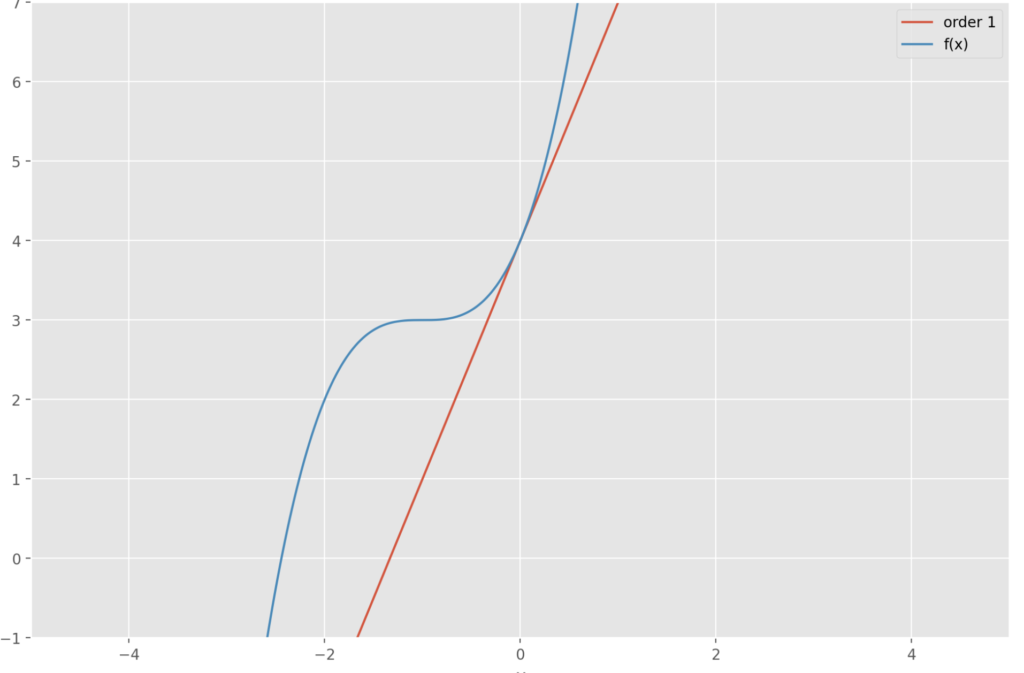
What happens if we take the derivative of p1(x) with respect to x? The constant term disappears, and the x in the second term disappears.

p_1'(x) = f'(0)

So the derivative of p1(x) for any point x is equivalent to the derivative of f'(0). That makes sense since p1 is a linear function. The slope must be the same everywhere. But a linear function is still not a good enough approximation. Now here is an interesting thought.

If setting the first derivative of p(x) equal to the first derivative of f(0) gives us a linear approximation, can we obtain higher-order approximations by making sure that higher-order derivatives of p(x) equal the corresponding higher-order derivatives of f(0)?

So if we can say that

p_2''(x) = f''(0)\\
p_3'''(x) = f'''(0)\\
etc.

can we construct a polynomial p(x) that equals f(x)?

Let’s try it out for the second derivative by constructing the second-order polynomial p2(x).

p_2(x) = f(0) + f'(0)x + \frac{1}{2} f''(0)x^2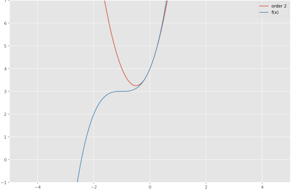

How did we arrive at this? Building on p1(x), we know that we need another second-order term x^2. We also know that the following expression needs to hold.

p_2''(x) = f''(0)

If we differentiate p2(x) two times, the first and zeroth-order terms will disappear. The second-order term x^2 will become 2. If we can turn the 2 into a 1, we are left with f”(0) as the only remaining expression on the right.

Likewise, we can construct the third order polynomial p3(x).

p_2(x) = f(0) + f'(0)x + \frac{1}{2} f''(0)x^2 +  \frac{1}{6} f'''(0)x^3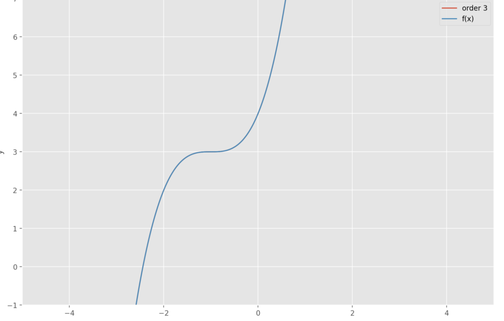

Differentiating three times, the first three terms disappear. Our third order term will become 6 as demonstrated in this helper function h(x).

h(x) = x^3\\
h'(x) = 3x^2\\
h''(x) = 6x\\
h'''(x) = 6\\

To arrive at

p_3'''(x) = f'''(0)\\

We need to put 1/6 in front of the third-order term.

In this case the function f(x) is a well behaved third order function. Accordingly, we attain a perfect approximation with a third order MacLaurin polynomial p3(x).

You can extend this process indefinitely until you arrive at the best possible approximation of your function. Accordingly, we can formalize the MacLaurin series.

p(x) = \sum\limits_{i=1}^\infty \frac{f^{n}(0)}{n!} x^n

Note: The exclamation mark is the mathematical symbol for factorial.

Taylor Series

The Taylor series can be considered a more general version of the MacLaurin series. While in the MacLaurin series we build our function around a point p for which x equals 0, the Taylor series allows us to build the function around any point p.

To construct the Taylor series, we start with a linear approximation p1(x) to our unknown function f(x). We know that the slope of p1(x) everywhere is equivalent to the slope of f(x) at the point p. Accordingly f'(p), the first derivative of f(x) at p, equals the slope of p1(x).

p_1(x) = f'(p)x + b

Furthermore, at point p, p1(x) and f(x) must be equivalent. Accordingly, we conclude the following.

f(p) = p_1(p)

f(p) = f'(p)p + b

With this knowledge, we can obtain the still unknown b as an expression of the other terms.

b = f(p) - f'(p)p

Now that we’ve gotten rid of the unknown constant b and replaced it with a generic expression in terms of p, we can reconstruct our original linear approximation function p1(x) with that generic expression.

p_1(x) = f'(p)x + f(p) - f'(p)p

Written in a more compact form:

p_1(x) = f(p) + f'(p)(x - p) 

Finally, we can apply the same logic used for the MacLaurin Series to create the Taylor series expansion to higher-order functions until we reach the best approximation to our function f(x).

p_2(x) = f(p) + f'(p)(x - p) + \frac{1}{2}f''(p)(x-p)^2 \\
p_3(x) = f(p) + f'(p)(x - p) + \frac{1}{2}f''(p)(x-p)^2 + \frac{1}{6}f'''(p)(x-p)^3\\
etc.

We can formalise the Taylor series in the following expression.

p(x) = \sum\limits_{i=1}^\infty \frac{f^{n}(p)}{n!} (x-p)^n

This post is part of a series on Calculus for Machine Learning. To read the other posts, go to the index.