What is Pooling in a Convolutional Neural Network (CNN): Pooling Layers Explained

Pooling in convolutional neural networks is a technique for generalizing features extracted by convolutional filters and helping the network recognize features independent of their location in the image.

Why Do We Need Pooling in a CNN?

Convolutional layers are the basic building blocks of a convolutional neural network used for computer vision applications such as image recognition. A convolutional layer slides a filter over the image and extracts features resulting in a feature map that can be fed to the next convolutional layer to extract higher-level features. Thus, stacking multiple convolutional layers allows CNNs to recognize increasingly complex structures and objects in an image.

A major problem with convolutional layers is that the feature map produced by the filter is location-dependent. This means that during training, convolutional neural networks learn to associate the presence of a certain feature with a specific location in the input image. This can severely depress performance. Instead, we want the feature map and the network to be translation invariant (a fancy expression that means that the location of the feature should not matter).

In the post on padding and stride, we discussed how a larger stride in convolution operations could help focus the image on higher-level features. Focusing on the higher-level structures makes the network less dependent on granular details that are tied to the location of the feature. Pooling is another approach for getting the network to focus on higher-level features.

In a convolutional neural network, pooling is usually applied on the feature map produced by a preceding convolutional layer and a non-linear activation function.

How Does Pooling Work?

The basic procedure of pooling is very similar to the convolution operation. You select a filter and slide it over the output feature map of the preceding convolutional layer. The most commonly used filter size is 2×2 and it is slid over the input using a stride of 2. Based on the type of pooling operation you’ve selected, the pooling filter calculates an output on the receptive field (the part of the feature map under the filter).

There are several approaches to pooling. The most commonly used approaches are max-pooling and average pooling.

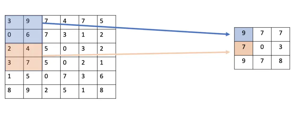
Max Pooling

In max pooling, the filter simply selects the maximum pixel value in the receptive field. For example, if you have 4 pixels in the field with values 3, 9, 0, and 6, you select 9.

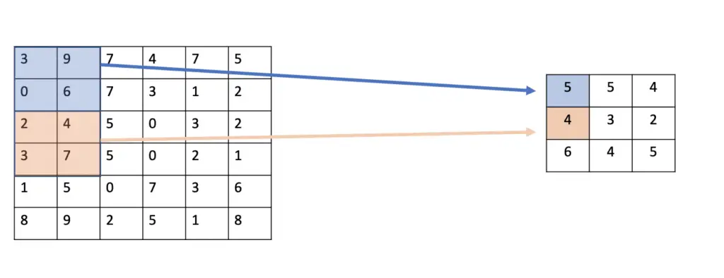
Average Pooling

Average pooling works by calculating the average value of the pixel values in the receptive field. Given 4 pixels with the values 3,9,0, and 6, the average pooling layer would produce an output of 4.5. Rounding to full numbers gives us 5.

Understanding the Value of Pooling

You can think of the numbers that are calculated and preserved by the pooling layers as indicating the presence of a particular feature. If the neural network only relied on the original feature map, its ability to detect the feature would depend on the location in the map. For example, if the number 9 was found only in the upper left quadrant, the network would learn to associate the feature connected to the number 9 with the upper left quadrant.
By applying pooling, we pull this feature out into a smaller, more general map that only indicates whether a feature is present in that particular quadrant or not. With every additional layer, the map shrinks, preserving only the important information about the presence of the features of interest. As the map becomes small, it becomes increasingly independent of the location of the feature. As long as the feature has been detected in the approximate vicinity of the original location, it should be similarly reflected in the map produced by the pooling layers.

Due to its focus on extreme values, max pooling is attentive to the more prominent features and edges in the receptive field. Average pooling, on the other hand, creates a smoother feature map because it produces averages instead of selecting the extreme values. In practice, max pooling is applied more often because it is generally better at identifying prominent features. In practical applications, average pooling is only used to collapse feature maps to a particular size.

Due to its ability to collapse feature maps, pooling can also help classify images of varying sizes. The classification layer in a neural network expects to receive inputs in the same format. Accordingly, we normally feed images in the same standard size. By varying the offsets during the pooling operation, we can summarize differently sized images and still produce similarly sized feature maps.

In general, pooling is especially helpful when you have an image classification task where you just need to detect the presence of a certain object in an image, but you don’t care where exactly it is located.
The fact that pooling filters use a larger stride than convolutional filters and result in smaller outputs also supports the efficiency of the network and leads to faster training. In other words, location invariance can greatly improve the statistical efficiency of the network.

This article is part of a blog post series on deep learning for computer vision. For the full series, go to the index.