Foundations of Deep Learning for Object Detection: From Sliding Windows to Anchor Boxes

In this post, we will cover the foundations of how neural networks learn to localize and detect objects.

Object Localization vs. Object Detection

Object localization refers to the practice of detecting a single prominent object in an image or a scene, while object detection is about detecting several objects.

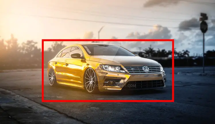
A neural network can localize objects in an image by learning to predict the coordinates of a bounding box around the object. A bounding box is simply a rectangular box around the object of interest. The network first performs a classification to predict whether the object of interest is present in the image. In addition to the classification, the network outputs the x and y coordinates of the center of the bounding box, as well as the width and height.

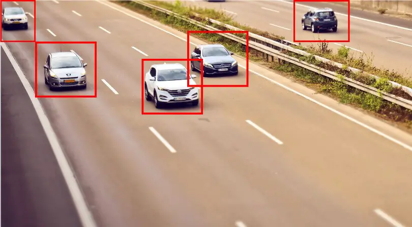
A neural network learns to detect multiple objects in an image using sliding windows. The sliding window algorithm slides multiple overlapping windows over the image of interest and detects whether an object of interest is present in the current area under the window. The network then relies on a metric called intersection-over-union to pick the best box and non-max suppression to discard boxes that are less accurate.

How to Find the Bounding Box

In a neural network trained for image classification, your last layer will use a sigmoid or softmax loss function to distinguish between two or more classes. The result will be a probability that the object belongs to a specific class. When performing object localization, we can extend a classification model by adding neurons to the network that also predict the location of the object of interest in the image.
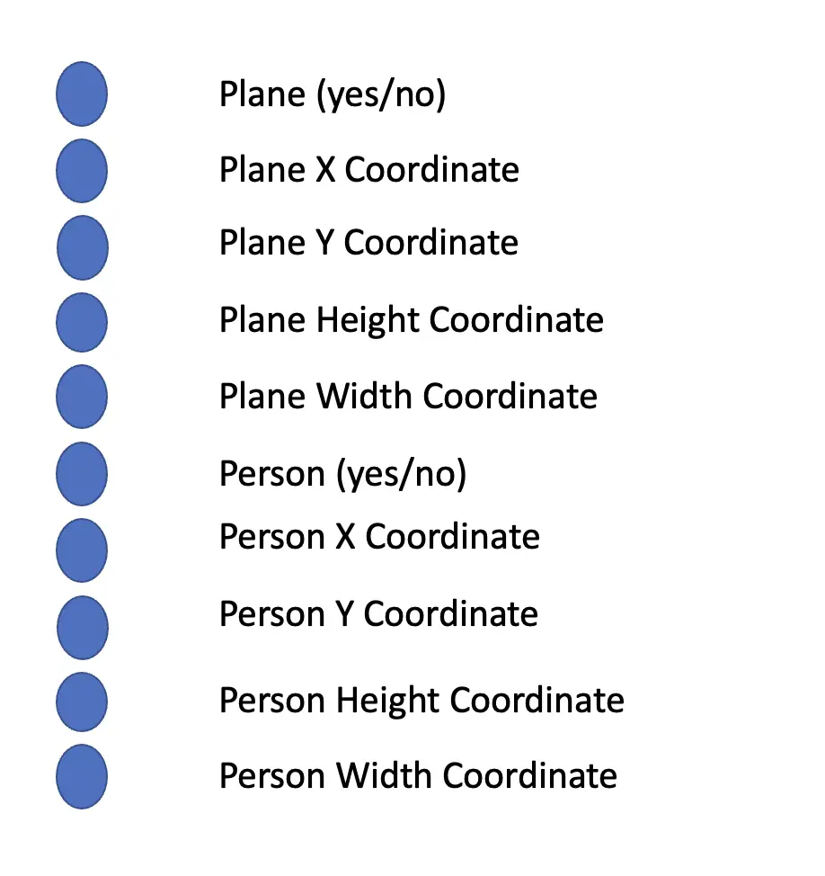
The standard way of representing the location of an object in the image is to draw a bounding box and have the neural network predict the x and y coordinates of the center of the box as well as its width and height.

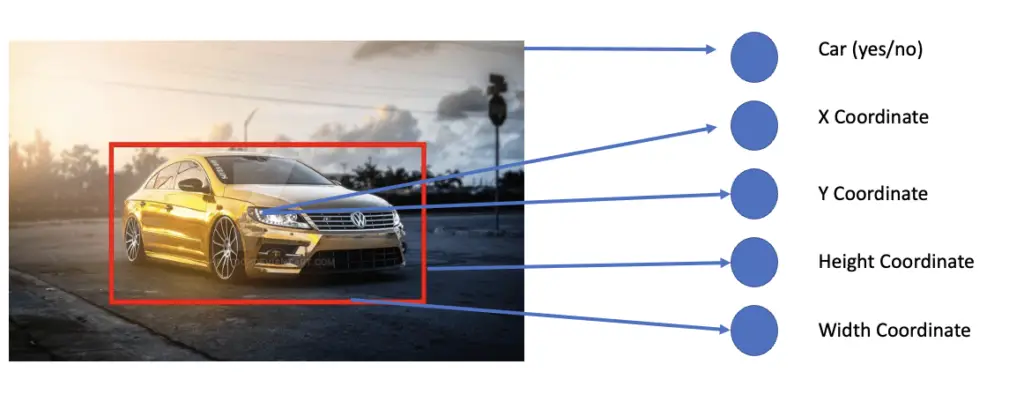
To teach the neural network to classify and localize the object, you have to provide it with the original images and the coordinates, height, and width of the bounding box.
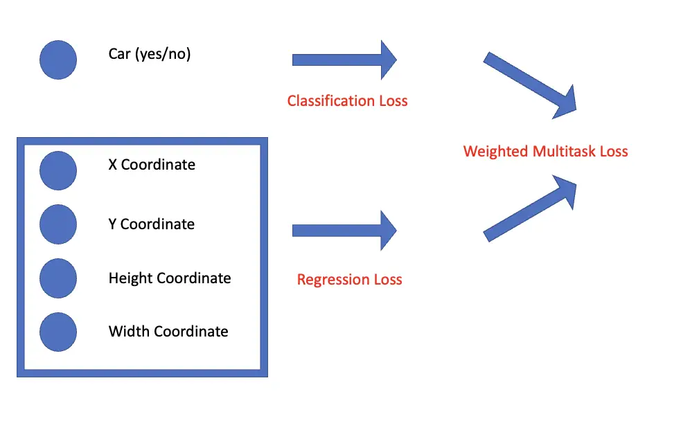
The network now has to perform two very different tasks at once. Determining the type of object is a classification task. Predicting the bounding box is a regression task because you need to quantify the difference between the predicted and the actual coordinates and box measurements.

As a consequence, you also need two different loss functions that you subsequently unify in a combined loss known as multitask loss. For the classification task, you use a loss function such as cross-entropy, while for the regression task, you use L2 loss or the intersection over union (a special kind of loss function for bounding boxes which we will cover in a later section).

Sliding Window Algorithm

As the name implies, the sliding window algorithm slides a window over some input array and applies an operation to the content under the window.
A classic example where the sliding window technique is useful would be finding the greatest sum of 2 consecutive elements in an array. To find that sum, we slide a window that encompasses exactly two numbers over the array and add the numbers together.

[1,2,3,4]
Window 1: [1,2] -> 3
Window 2: [2,3] -> 5
Window 3: [3,4] -> 7

The result equals 7.

In the case of images, we can use the sliding window to detect whether a feature or an object is present under the window.

Since an image is a 2-dimensional array, we have to slide the window horizontally and vertically. Each sub-image contained in a window is fed to a convolutional neural network which is used to classify whether an object of interest is contained in the image or not.

To increase the probability of finding an object of interest, you want to keep the stride (the size of the step between boxes) as small as possible. If you only advance your box by one pixel in each step, your stride would equal 1. The obvious disadvantage of this approach is that you will end up with almost as many boxes as there are pixels in the image. The computational cost would be prohibitively high, making this approach infeasible.

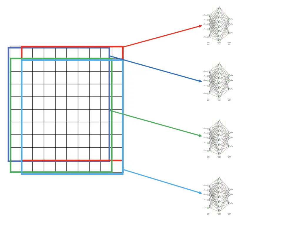
In the illustration above, we use a stride of 1 and a window size equivalent to the image size minus 1. As a consequence, we end up with 4 sliding windows. This is just for illustrative purposes. In a real implementation, the sliding window will likely be much smaller than the image, and you’ll end up with a lot more windows.

You can make this implementation a lot more efficient by making the sliding window convolutional. Instead of just applying a convolutional neural network to the single windows, you make the window extraction convolutional as well. The basic idea is that you apply a convolutional filter operation to the content under the sliding window and generate a feature map. If you are not sure how this works, check out my post on convolutional filters.

The convolutional operation will generate a feature map that is smaller than the original image by a factor of (filter size – 1). If we have a 10×10 input image and apply a 5×5 convolutional filter to it, the result should be a 6×6 feature map.

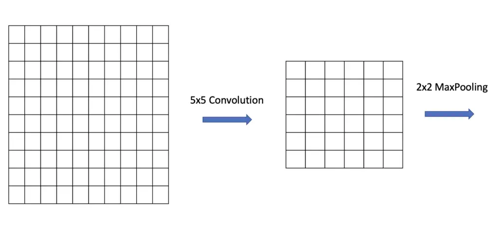
By applying Pooling with a 2×2 filter, we can cut the size of the feature map in half again to 3×3. After another convolution operation with a 2×2 filter, we end up with a 2×2 feature map.

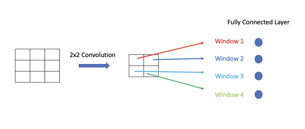
Each of the 4 windows in the feature map should now correspond to the 4 sliding windows in the original 10×10 image. Just like in a convolutional neural network, we can feed the outputs of the feature map to a fully connected layer and perform classification on it.

Instead of running 4 neural networks on each individual subwindow in succession, the convolutional implementation allows us to classify all windows in parallel through one neural network.

Intersection Over Union

Once the neural network has detected a bounding box, we need a way to evaluate how well the predicted bounding box corresponds to the ground truth bounding box. The method for quantifying the difference is known as intersection over union. The intersection over union measures the overlap between the areas of the predicted box and the ground-truth box. The formula, as the name implies, is a simple division of the area of the union of the two boxes, divided by the intersection of the two boxes.

 IoU = \frac{groundtruth\; \cap \;predicted }{groundtruth\; \cup \;predicted}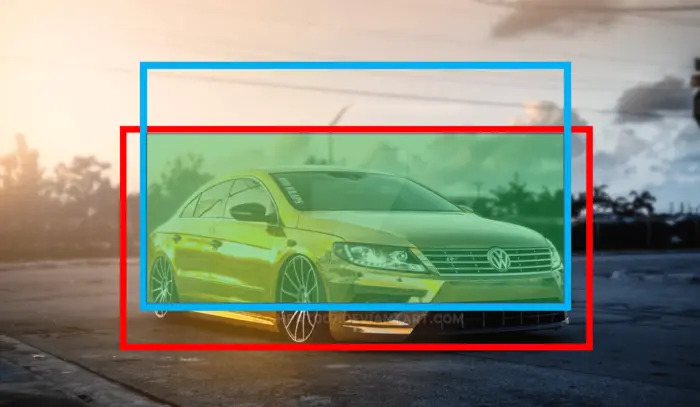

This formula gives you a ratio between 0 and 1. The larger that ratio, the more your predicted box overlaps with your ground truth box, and thus the more accurate your prediction. If you have several bounding boxes, the IoU enables you to choose the best box by picking the one with the highest ratio.
Conventionally, you want to aim for an IoU of at least 0.5.

Non-Max Suppression

When your sliding window moves over the image in small steps, it is likely that multiple windows will end up detecting the same object. It would be wasteful and confusing to produce multiple boxes therefore we rely on a technique known as non-max suppression to suppress all boxes except for the best.
When generating bounding boxes, the neural network will produce the coordinates of the box, as well as a confidence score that the box actually contains the desired object.
After the neural network has generated the bounding boxes, you use non-max suppression in the following way:

• Select the bounding box ‘a’ with the highest confidence score.
• Compare the proposal ‘a’ with the highest confidence with every other proposal by calculating the intersection over union.
• If the overlap between a and the other proposal is higher than a chosen threshold, remove the other proposal.
• Next, you choose the box with the highest confidence score out of the remaining boxes and repeat the process until no more boxes are left.

This process ensures, that for one area containing an object, there is only one significant bounding box.

Anchor Boxes

A major problem with the sliding-window based object detection mechanism is that each box can only contain one object. Anchor boxes allow us to detect multiple objects per window. To achieve the goal of multi-object detection, we need to define multiple anchor boxes depending on the number of objects we expect to detect. We also define the boxes with different dimensions to distinguish between objects of different shapes.

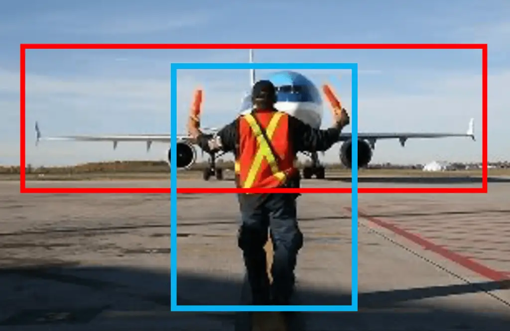
In the example above, we have two anchor boxes. This means you need to get your network to produce the classification for both objects in addition to the height, width of the box, and x, and y coordinates of the midpoint.

Now of course you may run into the problem that you have several anchor boxes assigned to a single object. To address this issue, you rely on the intersection over union again to calculate the overlap between the predicted bounding boxes and the ground truth.
Furthermore, the network detects the midpoint of the bounding box by finding the window that it deems to be closest to the midpoint of the object, and using the window’s midpoint. In rare cases, you may run into the problem that two bounding boxes have the same midpoint. But this shouldn’t happen if you keep the size of the windows relatively small.

This article is part of a blog post series on deep learning for computer vision. For the full series, go to the index.