Understanding Basic Neural Network Layers and Architecture

This post will introduce the basic architecture of a neural network and explain how input layers, hidden layers, and output layers work. We will discuss common considerations when architecting deep neural networks, such as the number of hidden layers, the number of units in a layer, and which activation functions to use.

In our technical discussion, we will focus exclusively on simple feed-forward neural networks for the scope of this post.

The Input Layer

The input layer accepts the input data and passes it to the first hidden layer. The input layer doesn’t perform any transformations on the data, so it usually isn’t counted towards the total number of layers in a neural network.

The number of neurons equals the number of features in the input dataset.

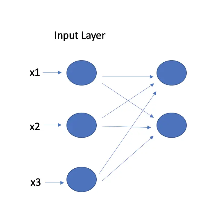
If you have multidimensional inputs, the input layer will flatten the images into one dimension. A network used for image classification requires images as input. A standard color RGB image usually has three dimensions: the width, the height, and three color channels. A greyscale image doesn’t need multiple color channels. Accordingly, two dimensions are sufficient. To feed a grayscale image to a neural network, you could transform every column of pixels into a vector and stack them on top of each other. A 4×4 grayscale image would thus require an input layer of 16 neurons.

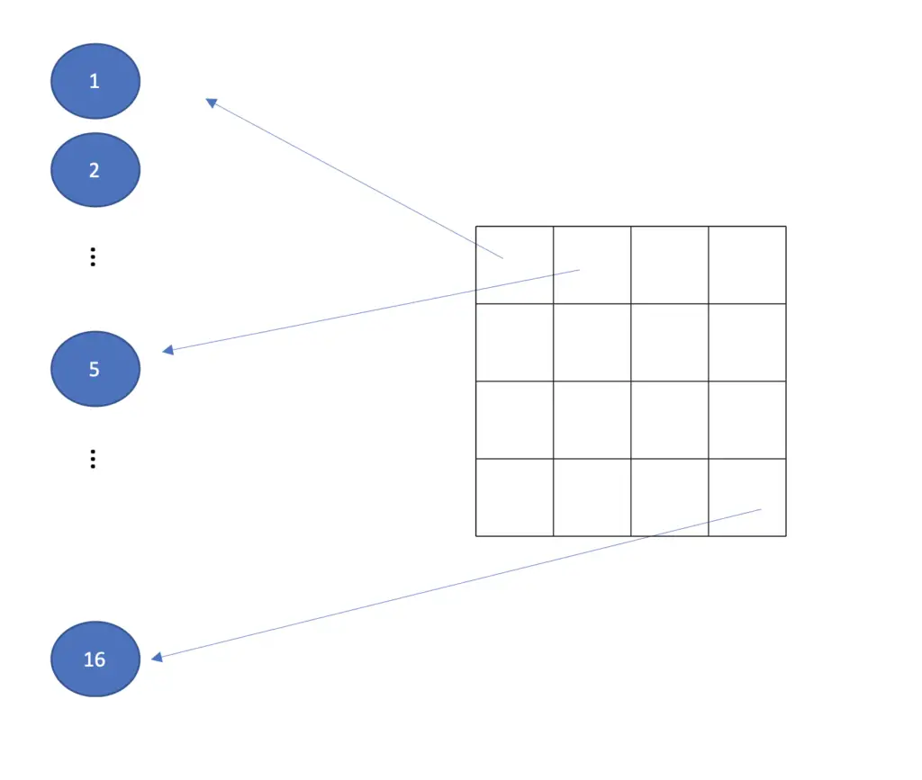
You could further flatten across the color channels given a color image. Modern deep learning frameworks usually take care of the flattening for you. You just need to pass the image to the input layer, specify its dimensions, and the framework will handle the rest.

The Hidden Layers

The goal of hidden layers is to perform one or more transformations on the input data that will ultimately produce an output that is close enough to the expected output. Hidden layers are where most of the magic happens that has put neural networks and deep learning at the cutting edge of modern artificial intelligence.

Why do Neural Networks Have Hidden Layers

The transformations performed by hidden layers can be fairly complex such as mapping from a piece of text in one language to its translation in another language. How would you represent the abstract relationship between a piece of text in English and its equivalent in Chinese in a mathematical function that captures the semantic meaning and context, grammatical rules, and cultural nuance?
More traditional machine learning algorithms perform rather poorly at tasks such as language translation because they cannot adequately represent the complexity of the relationship.
Neural networks excel at this type of task because you can get them to learn mappings of almost arbitrary complexity by adding more hidden layers and varying the number of neurons.

A neural network also has the advantage over most other machine learning algorithms in that it can extract complex features during the learning process without the need to explicitly represent those features. This allows a network to learn to recognize objects in images or structures in language. The hidden layers act as feature extractors. For example, in a deep learning-based image recognition system, the earlier layers extract low-level features such as horizontal and vertical lines. The later layers build on these extracted features to construct higher-level ones. Once you reach the output layer, recognizable objects should have been extracted so that the output layer can determine whether the desired object is present or not. The number of hidden layers depends on the complexity of the task and is usually found through experimentation.

What do Hidden Layers Compute

Hidden layers accept a vector of inputs from the preceding layer. Then they perform an affine transformation by multiplying with a weight term and adding a bias term.

z = W^Tx + b

Strictly speaking, the connections between the preceding layer and the current layer add the weight and the bias.

To capture non-linear relationships in a mapping, they then push the output z through a non-linear activation function.

a = f(z)

The deep learning research community has come up with several activation functions such as the rectified linear unit (ReLU), leaky ReLU, or the hyperbolic tangent function (Tanh). In the overwhelming majority of cases, the ReLU is a great default choice.

By chaining together several of these operations through multiple hidden layers, you can represent highly complex relationships.

The ReLU Activation Function

The ReLU activation simply returns the input when it is a positive number, and zero, when it is a negative number.

a = max(0, z)

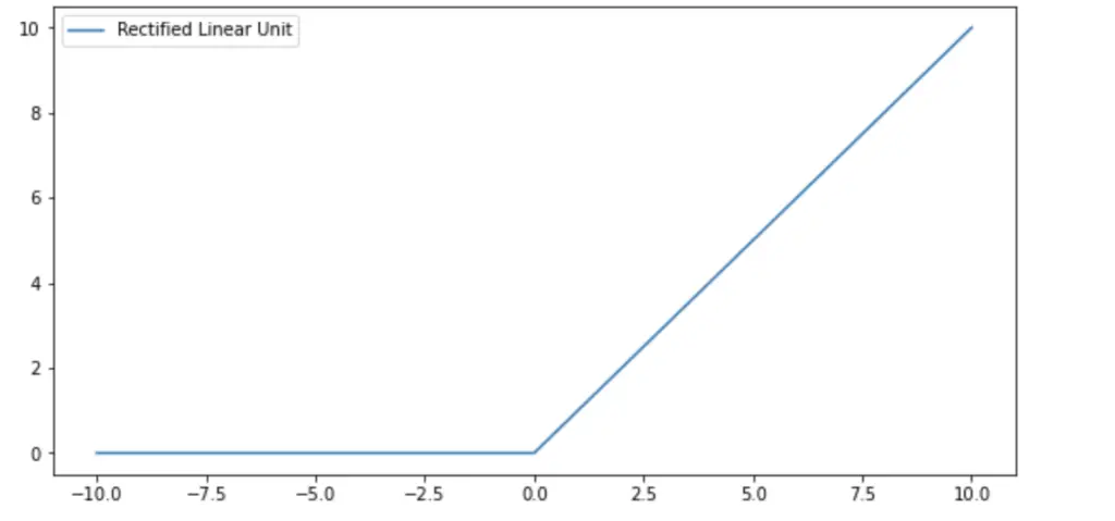
This looks very simple at first sight especially compared to other activation functions like the logistic sigmoid. But in the context of neural networks, the simplicity of the ReLU has several advantages.

• It is less computationally expensive to evaluate since there is no need for calculating exponentials.
• The previously applied sigmoid and TanH functions tend to saturate to either very high or very low values when the input is a huge positive or huge negative number. This leads to the problem of vanishing and exploding gradients. When you differentiate through these functions and through several layers, the gradient becomes so small or so large that it hinders the convergence of gradient descent. The ReLU performs a quasi-linear transformation. This prevents saturation and speeds up gradient descent.

How to Choose the Number of Hidden Layers

Generally speaking, more complex functions tend to require more layers to represent them appropriately. If you are dealing with a machine translation or image recognition task, you’ll need more layers than if you were classifying a patient as at risk for heart disease based on eating habits, age, and body mass index. The latter example is a simple classification task for which a neural network with one layer (logistic regression) would be sufficient. The former examples require multiple stages of hidden feature extraction and data transformation.

Unfortunately, there is no exact formula to determine the number of hidden layers in a neural network.

Your best bet is to study the standard networks implemented by the research community in your domain that achieve the best performance. This should give you a decent idea of how many layers and how many neurons are appropriate. Beyond that, you need to experiment systematically by tweaking network architectures and figure out what works best for your specific problem.

Types of Hidden Layers

In a simple multilayer perceptron, the hidden layers usually consist of so-called fully connected layers. They are called fully connected because each neuron in the preceding layer is connected to each neuron in the current layer.
In more advanced neural network architectures, you will find different types of layers.
The deep learning community has brought forth various layers for different purposes, such as convolutional layers and pooling layers in convolutional neural networks (primarily used in computer vision) or recurrent layers and attention layers in recurrent neural networks and transformers (mainly used in natural language processing). In future posts about more advanced neural network architectures for computer vision and natural language processing, I will discuss these layers.

The Output Layer

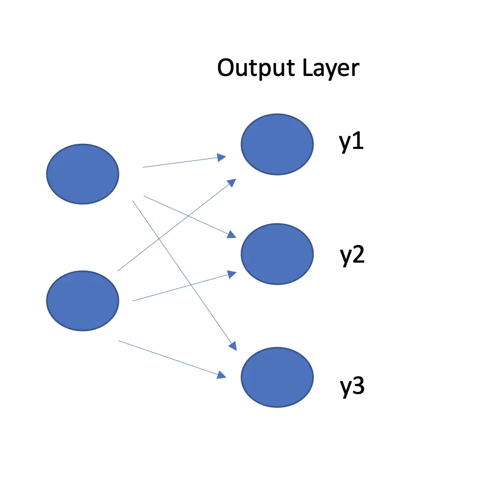
The output layer produces the final output computed by the neural network, which you compare against the expected output. The number of neurons in the output layer equals the number of classes the prediction can fall into.

For example, if your task was to classify whether an image contained a cat, a dog, or a rabbit, you would have three output classes and thus three neurons.

What does the Output Layer Compute

Much like the hidden layers, the output layer computes an affine transformation based on the weights and biases from the incoming connections.

z = W^Tx + b

Next, it applies a non-linear activation function that represents a probability value in a classification setting. This implies that the individual values need to be larger than zero but smaller than one, and all individual probabilities need to sum to one.

The most commonly used activation function in a binary classification setting is the logistic sigmoid, while in multiclass settings, the softmax is most frequently used.

Sigmoid and Softmax

The logistic sigmoid is an s-shaped function that asymptotes 0 as the input value z is negative, quickly grows towards one as z becomes positive, and asymptotes 1 with a growing positive z value.

\sigma(z) = \frac{1}{1+e^{-z}}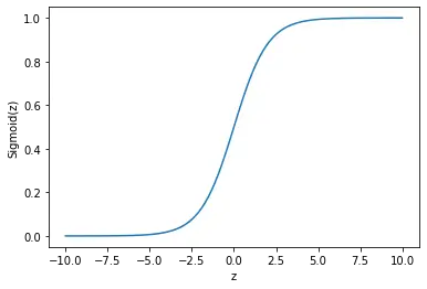

This makes it an ideal function for binary classification problems where the output can either be sorted into the class equivalent of 0 or 1.

The softmax function generalizes the sigmoid to a problem of an arbitrary number of k classes.

softmax(z) = \frac{e^{z(i)}}{\sum^k_{j=0} e^{z(j)}}

This article is part of a blog post series on the foundations of deep learning. For the full series, go to the index.