Understanding The Exploding and Vanishing Gradients Problem

In this post, we develop an understanding of why gradients can vanish or explode when training deep neural networks. Furthermore, we look at some strategies for avoiding exploding and vanishing gradients.

The vanishing gradient problem describes a situation encountered in the training of neural networks where the gradients used to update the weights shrink exponentially. As a consequence, the weights are not updated anymore, and learning stalls.

The exploding gradient problem describes a situation in the training of neural networks where the gradients used to update the weights grow exponentially. This prevents the backpropagation algorithm from making reasonable updates to the weights, and learning becomes unstable.

Why Do Gradients Vanish or Explode Exponentially?

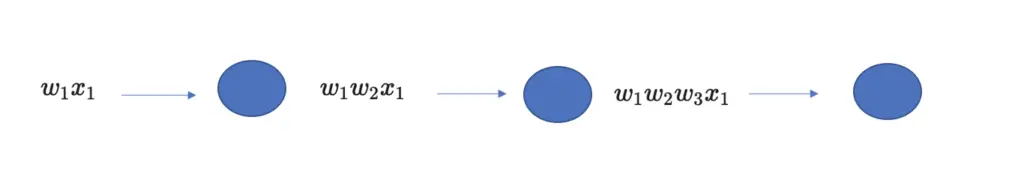
Suppose you have a very deep network with several dozens of layers. Each layer multiplies the input x with a weight w and sends the result through an activation function. For the sake of simplicity, we will ignore the bias term b.

a_1 =  \sigma(w_1x) \rightarrow a_2 = \sigma(w_2a_1) \rightarrow a_3 = \sigma(w_3a_2)

Further, suppose the activation function just passes through the term without performing any non-linear transformations. Essentially, every layer in the neural network just multiplies another weight to the current term.

Assume the weights are all equal to 0.6. This means with every additional layer; we multiply the weight by itself.

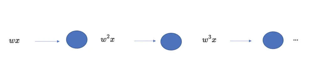
By the time you get to the third layer, you need to take the weight to the power of 3.

w^3 = 0.6^3 = 0.21

Now assume you have a network with 15 layers. Now your third weight equals w to the power of 15.

w^{15} = 0.6^{15} = 0.00047

As you can see, the weight is now vanishingly small, and it further shrinks exponentially with every additional layer.

The reverse is true if your initial weight is larger than 1, let’s say 1.6.

w^{15} = 1.6^{15} = 1152.92

Now, you have a problem with exploding gradients.

Every weight is actually a matrix of weights that is randomly initialized. A common procedure for weight initialization is to draw the weights randomly from a Gaussian distribution with mean 0 and variance 1. This means roughly 2/3 of the weights will have absolute values smaller than 1 while 1/3 will be larger than 1.

In summary, the further your values are from 1 or 0, the more quickly you run into either vanishing or exploding gradients when you have long computational graphs, such as in deep neural networks.

Vanishing and Exploding Gradients During Backpropagation

The previous example was mainly intended to illustrate the principle behind vanishing and exploding gradients and how it depends on the number of layers using forward propagation. In practice, it affects the gradients of the non-linear activation functions that are calculated during backpropagation.

Let’s have a look at an example using a highly simplified neural network with two layers.

During backpropagation, we move backward through the network, calculating the derivative of the cost function J with respect to the weights in every layer. We use these derivatives to update the weights at every step. For more detailed coverage of the backpropagation algorithm, check out my post on it.

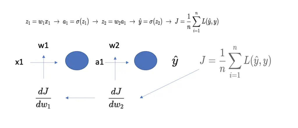
The derivatives are calculated and backpropagated using the chain rule of calculus. To obtain the gradient of the weight w2 in the illustration above, we first need to calculate the derivative of the cost function J with respect to the predicted value y hat.

\frac{dJ}{d\hat y}

Y hat results from the activation function in the last layer, which takes z2 as an input. So we need to calculate the derivative of Y hat with respect to z2.

\frac{d\hat y}{ dz_2} 

Z2 is a product of the weight w2 and the output from the previous layer a2. Accordingly, we calculate the derivative of u2 with respect to w2.

\frac{ dz_2} {dw_2}

Now we can calculate the gradient needed for adjusting w2, the derivative of the cost with respect to the w2, by chaining the previous three derivatives together using the chain rule.

\frac{dJ}{dw_2}  = \frac{dJ}{d\hat y} \frac{d\hat y}{ dz_2}  \frac{ dz_2} {dw_2}

Remember that the second gradient in the chain is the derivative of the activation function. Let’s assume we use the logistic sigmoid as an activation function. If we evaluate the derivative, we get the following result:

\frac{d\hat y}{ dz_2}  = \sigma(z_2)(1-\sigma(z_2)) =  \frac{1}{1 + e^{z_2}}( 1 -  \frac{1}{1 + e^{z_2}})

Let’s assume the value z2 equals 5. Evaluating the expression, we get the following:

\frac{d\hat y}{ dz_2}  = \sigma(5)(1-\sigma(5)) \approx 0.0066

As you see, the gradient is pretty small. If we have several of these expressions in our chain of derivatives, the gradient quickly shrinks to a number so small that it isn’t very useful for learning anymore.

To obtain the gradient of the first weight, we need to go even further back with the chain rule.

\frac{dJ}{dw_1}  = \frac{dJ}{d\hat y} \frac{d\hat y}{ dz_2} \frac{ dz_2} {da_1}\frac {da_1}{ dz_1} \frac {dz_1}{ dw_1}

Now we need to evaluate the derivatives of two activation functions. You can easily imagine what our gradient would look like if we had 15, 20, or even more layers and had to differentiate through all their respective activation functions.

How to Address Vanishing and Exploding Gradients?

Use the ReLU Activation Function

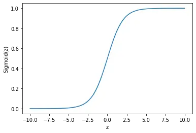
We’ve seen in the previous example that the sigmoid activation function is prone to creating vanishing gradients, especially when several of them are chained together. This is due to the fact that the sigmoid function saturates towards 0 for large negative or towards 1 for large positive values.

As you may know, most neural network architectures nowadays use the rectified linear unit (ReLU) rather than the logistic sigmoid function as an activation function in the hidden layers.

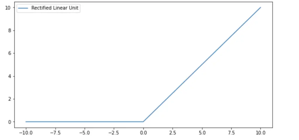
The ReLU function returns simply the input value if the input is positive and 0 if the input is negative.

f(z) =
\begin{dcases}
    0 \;for \; z < 0\\
    z \;for \; z \geq 0\\
\end{dcases}

The derivative of the ReLU is 1 for values larger than 0. This effectively addresses the vanishing gradient problem because multiplying 1 by itself many times over still gives you 1. You cannot differentiate the negative section of the ReLU function because it is 0. So as a convention, the derivative of negative values is just set to 0.

\frac{df(z)}{dz} =
\begin{dcases}
    0 \;for \; z < 0\\
    1 \;for \; z \geq 0\\
\end{dcases}

If you do need the negative section to be differentiable, you can use the leaky ReLU.

Weight Initialization

Another way to address vanishing and exploding gradients is through weight initialization techniques. In a neural network, we initialize the weights randomly. Certain techniques such as He initialization and Xavier initialization ensure that the weights are close to 1.

For every layer, weights are commonly sampled from a normal distribution with a mean of 0 and a standard deviation equal to 1.

\mu = 0 \;and\; \sigma = 1

This results in weights that are all over the place in a range from roughly -3 to 3.

He initialization samples weights from a normal distribution with the following parameters for mean and standard deviation, where n is the number of neurons in the preceding layer.

\mu = 0 \;and\; \sigma = \sqrt{\frac{1}{n_{l}}} \;or\; \sigma = \sqrt{\frac{2}{n_{l}}}

Xavier initialization uses the following parameter for weight initialization:

\mu = 0 \;and\; \sigma = \sqrt{\frac{2}{n_{l} + n_{l+1}}}

The adjusted standard deviation helps constrain the weights to a range that makes exploding and vanishing gradients less likely.

Gradient Cliping

Another simple option is gradient clipping. This way, you just define an interval within which you expected the gradients to fall. If the gradients exceed the permissible maximum, you automatically set them to the maximum upper bound of your interval. Similarly, if they fall below the permissible minimum, you automatically set them to the lower bound.

This article is part of a blog post series on the foundations of deep learning. For the full series, go to the index.