An Introduction to Autoencoders and Variational Autoencoders

What is an Autoencoder?

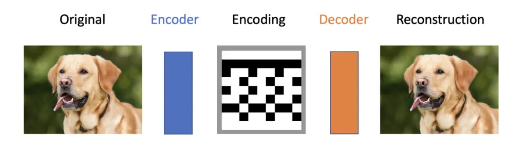
An autoencoder is a neural network trained to compress its input and recreate the original input from the compressed data. This procedure is useful in applications such as dimensionality reduction or file compression where we want to store a version of our data that is more memory efficient or reconstruct a version that is less noisy than the original data.

Autoencoders consist of two main components to achieve the goal of reconstructing data:

• an encoder network that learns to create a compressed or encoded version of the input data.
• a decoder network that is trained to reconstruct the original data from the compressed version.

Mathematically, we can describe the encoder as a function f that takes an input x to create an encoding h.

h = f(x)

The decoder represents another function, d that takes h as an input to produce a reconstruction r.

r = d(h)

Essentially, the autoencoder is trained to learn the following mapping:

r = d(f(x))

As you can see, the autoencoder does not learn to exactly reconstruct the original input x but r, which is an approximation to x.
An important feature of autoencoders is that they are unable to learn the identity function and reconstruct the original input perfectly. Instead, they are designed in a way that only allows for approximate recreations.
If we allowed an autoencoder to reconstruct the original image, it might default to just learning the identity function. Then the encoding will look exactly like the input making the autoencoder essentially useless.

The hidden layers have fewer nodes than the input and output layers to prevent the networks from learning the identity function. The number of nodes in the output layer equals the number of nodes in the input layer to allow for a reconstruction that is similar to the original.

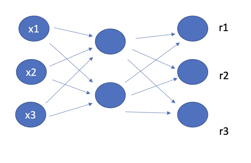
Reducing the number of hidden nodes available to fewer than the input forces the autoencoder to prioritize the features it wants to preserve. These features need to be useful for reconstruction, which induces the network to focus on useful properties and ignore the noise.
Let’s say we wanted to build an autoencoder to encode and reconstruct an image of 20×20 = 400 pixels. Since we don’t use convolutions, we require 400 neurons in the input and output layers. If we equipped the hidden layers with 400 neurons as well, the autoencoder could simply pass through the single pixels without learning anything about the relationship between the pixels. Let’s cut the number of neurons in the hidden layers down to 200. Now, the network is forced to learn a useful representation of the 400 pixels it receives from the input layer that can be processed by 200 neurons and which allows for a reconstruction of the full 400 pixels that is as accurate as possible.
We call networks, which do not have the capacity to learn the full mapping, under-complete. As we discuss later in this article, there are other ways to force autoencoders to not learn the full mapping.

Compared to deterministic methods for data compression, autoencoders are learned. This means they rely on features that are specific to the data that the autoencoder has been trained on. An autoencoder will perform poorly with data it hasn’t been trained on.

What is a Variational Autoencoder?

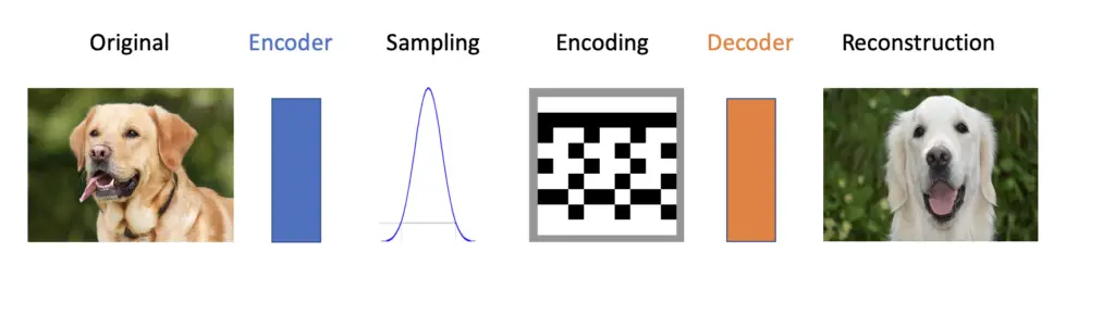
A variational autoencoder, in contrast to an autoencoder, assumes that the data has been generated according to some probability distribution. The variational autoencoder tries to model that distribution and find the underlying parameters. Learning a probability distribution allows variational autoencoders to not only reconstruct data but to generate new data on the basis of that distribution.

To build a variational autoencoder in practice, we still encode the data using an encoder network. But instead of creating an encoding straight from the output of the encoder, we use the output to parameterize a Gaussian distribution. To generate the encoding, we sample the data from that distribution. The decoder then learns to recreate the image from the encoding. Due to the stochasticity inherent in the sampling process and thus in the encoding, the reconstruction will be similar but different from the original. For example, if you feed an image of a dog to the autoencoder, the reconstruction should be a different dog.

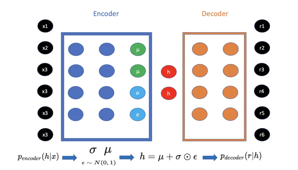
Mathematically, instead of defining the encoder as a function mapping x to a lower-dimensional encoding h, we define it as a conditional probability distribution that produces h given x.

p_{encoder} (h |x)

Similarly, we define the decoder as producing r given the encoding h.

p_{decoder}(r|h)

In practice, you

• feed your input x (such as an image) to the encoder
• train your encoder to produce μ and σ, the parameters of a Gaussian distribution. A Gaussian distribution is parameterized by a mean (μ) and a standard deviation (σ)
• randomly sample a term ε from a standard Gaussian distribution (with mean 0 and standard deviation 1)

\epsilon \sim N(0, 1) 

• create the latent encoding vector h by multiplying σ with the randomly sampled ε and adding it to the mean μ. This creates the stochasticity that enables the variational autoencoder to generate new data. Note that there are different versions of this formula.

h = \mu + \sigma \odot \epsilon

• Lastly, you pass h to the decoder which produces r in an attempt to recreate x.

Autoencoder Loss Functions

Just as other neural networks, autoencoders use cost functions to measure the reconstruction loss and reduce it through backpropagation with gradient descent.

The goal of the autoencoder is to reduce the loss between the original input x and the reconstruction r that has been generated by the encoder f and the decoder d.

L(x, r) = L(x, d(f(x)))

Several loss functions are applicable to variational autoencoders.

Mean Squared Error

The mean squared error usually works pretty well in vanilla autoencoders. It measures the squared distances between an observation in x and in r.

L(x_i,r_i) = || x_i -r_i||^2

The cost across the entire dataset is the sum of the squared distances between the observations in x and r.

J(x, r) = \frac{1}{n}\sum^n_{i=1} (x_i - r_i)^2

Binary Cross Entropy

If your data is binary or at least in the range [0,1], you can also use binary cross-entropy in vanilla autoencoders.

J(x, r) = - \sum^n_{i=1} x_i log(r_i) + (1-x_i) log(1-r_i)

Variational Autoencoder Loss and Kullback Leibler Divergence

When training variational autoencoders, we do not aim to reconstruct the original input. Instead, the goal is to generate a new output that is reasonably similar to the input but nevertheless different. Accordingly, we need a way to quantify the degree of similarity rather than the exact difference. We can achieve this by measuring the difference between the probability distributions underlying the data generating process of the input and the output.

As the name implies, the Kullback-Leibler divergence measures the divergence between 2 probability distributions, P and Q.

D_{KL}(P || Q)

In a discrete data setting, the Kullback-Leibler divergence is calculated as follows:

D_{KL}(P||Q) = \sum_{i=1}^n P(x_i) log(\frac{Q(x_i)}{P(x_i)})

P(x) represents the distribution of the encoder p_{encoder} (h |x) that projects our input variable x into latent space to create the encoding h. As discussed in the section above, when training a variational autoencoder, we let the encoder produce the parameters σ and μ of a normal distribution.

The standard normal distribution is our prior distribution p(h) if we don’t know anything about the input data. To quantify the loss, we measure the divergence of p_{encoder} (h |x) from a standard normal distribution using the Kullback-Leibler divergence.

D_{KL}(p_{encoder} (h |x) || p(h)) =  D_{KL}(N(\mu, \sigma) || N(0,1)) 

In practice, we plug the values generated by the encoder into a derivation of the Kullback Leibler divergence for Gaussian distributions.

D_{KL}(p_{encoder} (h |x) || p(h)) = 

\frac{1}{2}\left[-\sum_i\left(\log\sigma_i^2 + 1\right) + \sum_i\sigma_i^2 + \sum_i\mu^2_i\right]

The derivation goes beyond the scope of this post. If you are interested in it, here is the derivation in a post on Stats Stackexchange.

To calculate the full variational autoencoder loss, we calculate the loss between the original input and the reconstruction. Then we add the Kullback Leibler divergence between the probability distributions underlying the data generating process of the input and the output.

L = \frac{1}{n}\sum^n_{i=1} (x_i - r_i)^2 +  \frac{1}{2}\left[-\sum_i\left(\log\sigma_i^2 + 1\right) + \sum_i\sigma_i^2 + \sum_i\mu^2_i\right]

Autoencoder Regularization

Autoencoders with an equal or higher number of neurons compared to the input layer have too much capacity and are known as overcomplete. As previously stated, we usually design autoencoders to be under-complete. By giving the hidden layers fewer neurons and thus less capacity, we prevent the autoencoder from simply copying the input to the output without learning anything about the underlying structure in the data.
In addition to the number of neurons in the hidden layers, the capacity of an autoencoder also depends on the number of hidden layers or depth of the network. Designing the capacity of autoencoders and variational autoencoders to fit the complexity of the data distribution is one of the major challenges in training those networks.

Regularization techniques can help us prevent an autoencoder from simply copying its input to its output, even in the over-complete case. Thus, regularization allows us to add more capacity to models by increasing their depth and breadth while enabling them to learn useful mappings.

Note that variational autoencoders are trained to maximize a probability distribution given the input data rather than learning to reconstruct the data directly. Remember that the generation of the encodings involves a random term. Accordingly, a variational autoencoder cannot learn a deterministic identity function which is why regularization is not necessary.

Sparse Autoencoder

Sparsity in the context of neural networks means that we deactivate neurons and thus prevent them from transmitting an impulse. The underlying idea is that if we enforce a sparsity constraint on the hidden layers in an autoencoder, it shouldn’t be able to learn the identity function even if the layer is large.

Standard activation functions such as the logistic sigmoid constrain the impulse to a value between 0 and 1. Generally speaking, if the output of a neuron is close to 0, it won’t transmit an impulse, while if it’s close to 1, it will. In a sparse layer, we want many of the neurons to have outputs close to 0 to prevent them from firing.

One way to enforce sparsity on the hidden layer is to penalize the average activations in the hidden layer through the cost function. Using the L1 norm, we can add a regularization term Ω that is a function of the encoding layer h and has the effect of shrinking many of the parameters in h to 0. With the hyperparameter λ, we can control the regularizing effect.

J(x, r) = \frac{1}{n}\sum^n_{i=1} (x_i - r_i)^2 + \lambda \Omega(h)

If you don’t know why L1 regularization can set parameters equal to 0, check out my post on regularization in machine learning.

An approach that is described in detail in this Stanford lecture enforces a penalty using the average activations in the hidden layer. The idea is that in a hidden layer you want to make sparse, the average activation \hat p across all neurons should be relatively small because most neurons produce no impulses. So you can set a relatively small target value p and use a measure of the difference as a penalty on the cost function. If many neurons in the hidden layer are active, the average activation will be relatively large, and thus the penalty on the cost is larger as well.

Denoising Autoencoder

Denoising autoencoders work by corrupting the input source of the data. The autoencoder is then trained to reconstruct the original data from the corrupted input. For example, if you are training an autoencoder to reconstruct pictures from photos that have been blurred.

If x is our original input data, and \hat x is the corrupted version of x, the denoising autoencoder is trained to reduce the following loss:

L(x, r) = L(x, d(f(\hat x)))

Why Make Autoencoder Deep?

The ability of neural networks to learn complex mappings can generally be improved by either increasing the number of neurons in the layers, or by increasing the number of layers. Since autoencoders consist of feedforward networks, the same reasoning applies to them.
In general, increasing the number of layers and thus making the network deeper as opposed to simply adding more neurons, can dramatically reduce the computational cost and training data required for learning certain functions. If you are interested in why that is the case, check out this paper.
It has also been determined experimentally that deep autoencoders are better at compressing data than shallow ones.

This article is part of a blog post series on deep learning for computer vision. For the full series, go to the index.