Student’s T-Distribution

In this post we introduce student’s t-distribution and learn how to construct t-confidence intervals.

The t distribution is usually applied when you want to estimate the mean of normally distributed data but the sample size is small and you don’t know the population standard deviation. Like the Chi-Square distribution, it relies on degrees of freedom to account for the volatility inherent in a small sample size.

How does that volatility play out?

T Distribution Formula

Remember the formula for the Z-score.

Z_n = \frac{\bar X_n - \mu}{\frac{\sigma}{\sqrt{n}}} 

Since the sample size is large, we simply put the value for the sample standard deviation in place of the population standard deviation because they are sufficiently close to each other.

With a small sample size the sample standard deviation is likely to deviate more strongly from the population standard deviation. So in case of the t-distribution, we need to work explicitly with the sample standard deviation s.

t_n = \frac{\bar X_n - \mu}{\frac{s}{\sqrt{n}}}

In practice, this means the t distribution will look like the normal distribution but have higher variance the fewer observations n your sample has. The t distribution has (n-1) degrees of freedom.

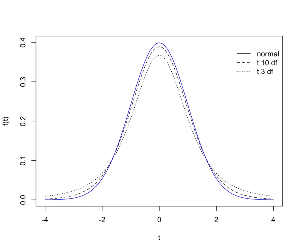
As the sample size gets larger, the t-distribution approximates the standard normal distribution.

Mathematically, the t-distribution is the standard normal variable z divided by the Chi-Square X^2

T = \frac{Z}{\sqrt{\Chi^2/(n-1)}}

The square root of the Chi-Square divided by its degrees of freedom simplifies to the sample standard deviation divided by the population standard deviation.

\sqrt{\frac{\Chi^2}{n-1}} = \frac{s}{\sigma}

Given this knowledge, we can easily derive the t distribution.

t = \frac{\frac{\bar X - \mu}{\sigma/\sqrt{n}}}{ \frac{s}{\sigma}} =  \frac{\bar X - \mu}{\frac{s}{\sqrt{n}}}

T Confidence Interval

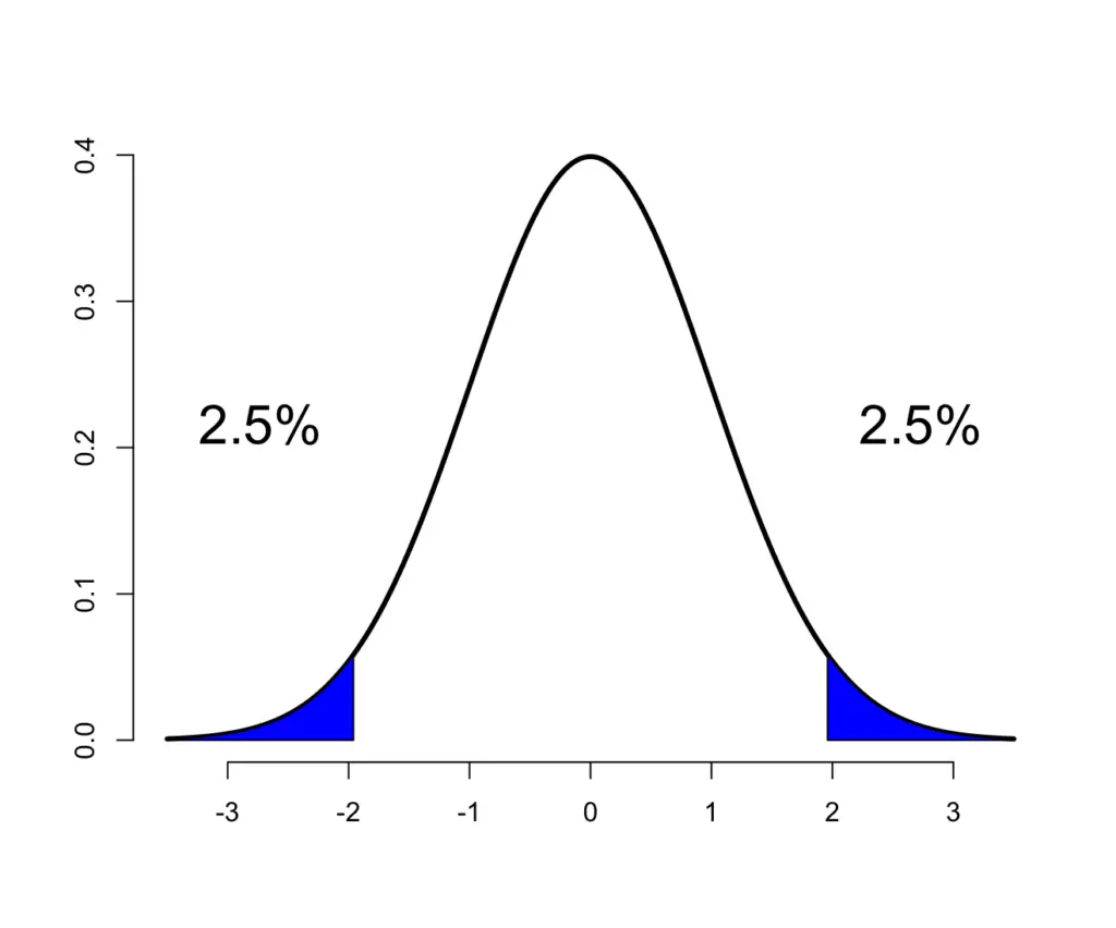
Now that we have the formula for the t-statistic we can construct a confidence interval for the mean of normally distributed data. First, we need to choose a significance level α. We choose the standard 5% so our confidence interval 1-α encapsulates 95% of our data. For a two-sided interval, we are interested in two critical points t and -t that mark the lowest 2.5% and the highest 2.5% of our data. Once you know the confidence level and the degrees of freedom, you can look up the t value in a t-distribution table.

Our mean T must fall between the two values t, -t with a confidence of 1-α (95%).

1- \alpha = P(-t_{alpha/2} < T < t_{alpha/2})

1- \alpha = P(-t_{alpha/2} < \frac{\bar X - \mu}{\frac{s}{\sqrt{n}}} < t_{alpha/2})

With a little bit of algebraic transformation, we arrive at a practical formula for calculating the confidence interval.

P(\bar X -t_{alpha/2} \frac{s}{\sqrt{n}} <  \mu < \bar X + t_{alpha/2} \frac{s}{\sqrt{n}})

In a previous post on confidence intervals, we used the z-score to estimate the mean. In practice, the t confidence interval is a more appropriate fit regardless of the sample size. That is because as the sample size increases, the t distribution approximates the normal distribution.

T Confidence Interval Example

Let’s do an example to make this clearer. A school is planning to introduce a new test and wants to make sure it is neither too easy nor too difficult. Unfortunately, they could only do a trial run on a sample of n=10 students who had a mean score X of 66 on a test and a standard deviation of 15. We want to find the two-sided 95% confidence interval for the true sample mean.

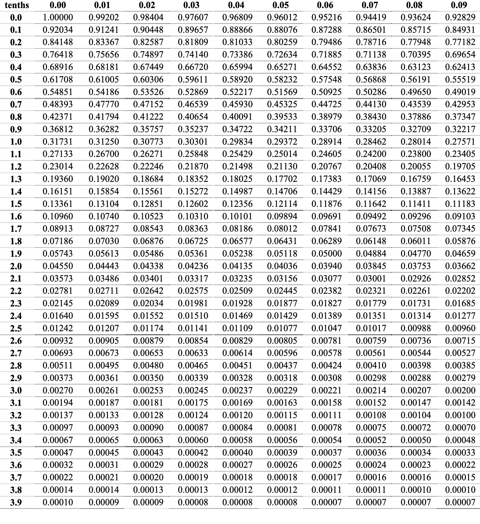
First, we look up the degrees of freedom from the t-table. We have 9 degrees of freedom

(n-1) = (10-1) = 9 

and we need the 2.5th percentile since we are doing a 2-sided test.

Our t- value is

t_{0.025, df=9} = 2.262

Now, we can plug this into our formula:

\bar X + t_{alpha/2} \frac{s}{\sqrt{n}} = 66 + 2.262 \frac{15}{\sqrt{10}} = 76.73

\bar X - t_{alpha/2} \frac{s}{\sqrt{n}} = 66 - 2.262 \frac{15}{\sqrt{10}} = 55.27

We are 95% confident that our true mean score on the test will lie between 55.27 and 76.73. We’ll leave it to the principal and the teachers to decide whether the test is too difficult or too easy or just right.

Probability Density Function of The T-Distribution

The pdf of the T-distribution isn’t used very much in practice. For completeness, I’ll give you the formula. It is essentially a combination of the gamma distribution and the normal distribution.

f(t) = \frac{\Gamma((n+1)/2)}{\sqrt{\pi t} \Gamma(r/2)} \frac{1}{(1+t^2/r)^{(r+1)/2}}

This post is part of a series on statistics for machine learning and data science. To read other posts in this series, go to the index.