Ordinary Least Squares Regression

In this post, we are going to develop a mathematical understanding of linear regression using the most commonly applied method of ordinary least squares. We will use linear algebra and calculus to demonstrate why the least-squares method works.

For a simple, intuitive introduction to regression that doesn’t require advanced math, check out the previous post on the least-squares regression line.

Simple Linear Regression Model

With simple linear regression, we can linearly model the relationship between an explanatory variable x, and a predicted response variable y. For example, you could model how height predicts the weight of a person.

In its simplest form, a linear regression model is a line with an intercept α, α slope β, and an error term ε, which describes how far the line deviates from the actual observations, the predictor variable x, and the predicted variable y.

Simple Linear Regression Formula

A single observation y_i is predicted according to the following equation.

y_i = \alpha + \beta x_i + \epsilon_i 

Since x and y consist of multiple observations n, we describe them as vectors with n entries. Epsilon measures the difference between every single, observation and its predicted value on the regression line. Accordingly, it also needs to be described in vector form with n entries.

\{x_i, y_i\, \epsilon_i \}^n_{i=1}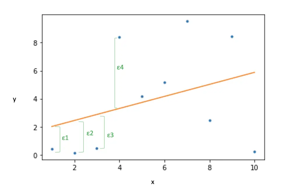

If we fully write out the vectors, our simple regression model looks like this:

\begin{bmatrix}  
y_1\\
y_2\\
... \\
y_n
\end{bmatrix} 
 = \alpha + 
\beta \begin{bmatrix}  
x_1\\
x_2\\
... \\
x_n
\end{bmatrix} 
+
\begin{bmatrix}  
 \epsilon_1\\
 \epsilon_2\\
... \\
 \epsilon_n
\end{bmatrix} 

Ordinary Least Squares

Using a least-squares approach, our goal is to minimize the sum of the squared errors, the distances of single data points from the line.

We first rearrange our linear regression equation for a single value to express the errors.

  \epsilon_i = y_i - \alpha - \beta x_i

The minimum values for α, β, and ε which we denote as follows.

\{\hat a, \hat \beta, \hat \epsilon\}

We actually want to find the sum of all squared errors that minimize this expression. We denote this expression with S.

S = \sum_{i=1}^n \epsilon^2_i = \sum_{i=1}^n (y_i - \alpha - \beta x_i)^2

From calculus, we know that at its minimum value, a function has a slope of zero. To find the values α, β that minimize ε^2 we have to differentiate S with respect to α, and β and set theses expression equal to zero. This gives us a so-called Jacobian vector that contains our derivatives.

\begin{bmatrix}
    \frac{\partial{S}}{\partial{\beta}} \\
     \frac{\partial{S}}{\partial{\alpha}}
  \end{bmatrix}

= 

\begin{bmatrix}
    0 \\
     0
  \end{bmatrix}
=

\begin{bmatrix}
    2 \sum_i x_i(y_i - \alpha - \beta x_i) \\
      2 \sum_i (y_i - \alpha - \beta x_i) 
  \end{bmatrix}

We can easily arrive at the expression for our minimum α hat by summing out the second equation and dividing by the number of data points n. We now have averages of α, β rather than sums of single values. Since the left part of the equation is zero, we can also get rid of two by simply dividing by two.

Thus, we arrive at a final expression for the minimum α where y and x with the bar on top denote the average values across all n datapoints.

\hat \alpha = \bar y - \beta \bar x

We can apply a similar transformation to the first equation arriving at the following expression for minimum β.

\hat \beta = \frac{\sum(x-\bar x)y}{\sum(x-\bar x)^2}

This is equivalent to the sample covariance divided by the sample variance.

\hat \beta = \frac{Cov(x,y)}{Var(x)}

Multiple Linear Regression Model

In multiple linear regression, you have more than one explanatory variable. For example, body weight is probably not only predicted by weight. In a multiple linear regression setting, you could add more predictors such as age, and calories consumed per day.

Mathematically, we write the multiple regression model with k predictors as follows:

y_i = \beta_0 + \beta_1 x_{i1} + \beta_2 x_{i2} + ... + \beta_k x_{ik} + \epsilon_i

Remember, i denotes a single observation, whereas k is the number of predictors. This implies, that every observation becomes a vector of k entries over all predictors.

Multiple Linear Regression Formula

The equation for a single entry looks like this.

y_i = x_i^T \beta + \epsilon_i

Note, that we have to transpose the vector x_i to take its inner product with beta.

x_i = [x_{i1}, x_{i2}, ...,x_{ik}]^T

Now we can write the predictors as a matrix X, our beta as a vector; and we can take the inner product.

X = \begin{bmatrix}  
x_{11} & ... & x_{1k} \\
... & ... & ...\\
x_{n1} & ... & x_{nk}
\end{bmatrix} \;
\beta = 
\begin{bmatrix}  
\beta_0 \\
...\\
\beta_k \\
\end{bmatrix}

The whole regression equation can be written in succinct matrix notation where X is a matrix and y, β, ε are vectors:

y = X\beta+\epsilon

To find the values that minimize ε, the process is the same as with simple linear regression. We find the squared difference between the Xβ and y.

S =  \left \| y - X\beta  \right\|^2 = (y-X\beta)^T(y-X\beta)

S = y^Ty - 2y^TX\beta+\beta^TX^TX\beta

We want to minimize beta. So, we take the derivative of S with respect to beta and set it equal to zero.

\frac{\partial S}{\partial \beta} = - 2X^Ty + 2X^TX\beta = 0

Finally, we divide by two and rearrange terms to express β minimum.

\hat\beta = (X^TX)^{-1}X^Ty

To find beta, we can multiply y with this matrix expression of X, known as the Moore-Penrose Pseudoinverse.

(X^TX)^{-1}X^T

Summary

We’ve looked at a mathematical introduction to simple linear regression and multiple linear regression using ordinary least squares.