Introducing Variance and the Expected Value

In this post, we are going to look at how to calculate expected values and variances for both discrete and continuous random variables. We will introduce the theory and illustrate every concept with an example.
Expected Value of a Discrete Random Variable
The expected value of a random variable X is usually its mean. The outcome of X is defined by a probability distribution p(x) over the concrete values x = \{x1,x2,...,xn\} that X can assume.
You can calculate the mean or expected value of a discrete random variable X by
- multiplying each value in x by its probability as defined by p(x)
- summing overall x p(x)
E(X) = \sum_x xp(x)
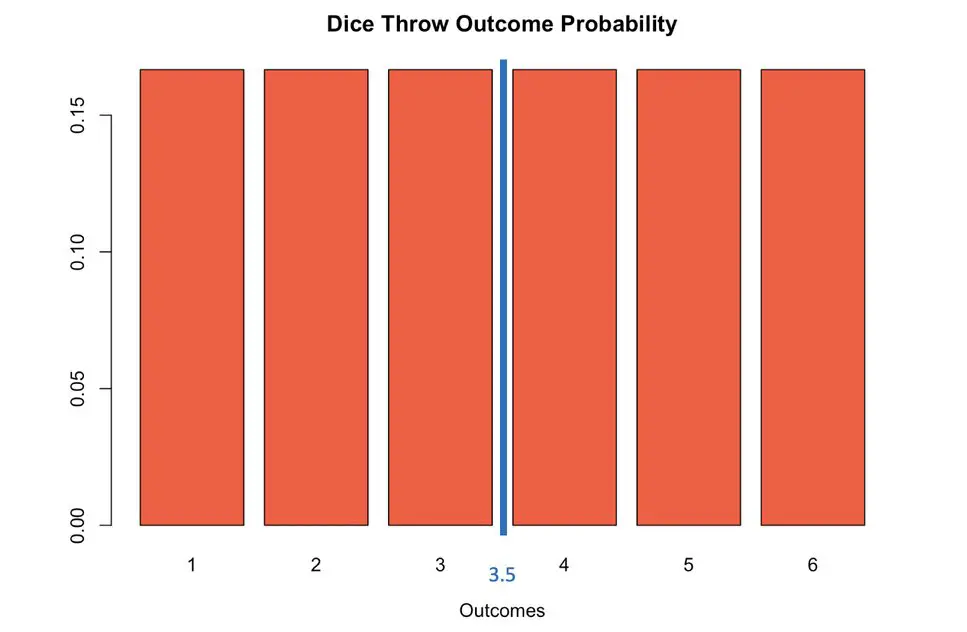
This was fairly abstract. To build the intuition, let’s suppose you are throwing a six-sided fair dice. We have the following values for x.
x = \{1,2,3,4,5,6\}Each value has a probability of 1/6 of being the result of a dice throw.
If you throw the dice once, it could return any number. However, if you throw a dice many times you’d expect every value from one to 6 to come up with approximately the same frequency. If you took the average of all the results and divided it by the number of throws, you’d expect it to return the geometric mean between 1 and 6, which is 3.5.
We can now calculate our expected value as follows. This should give us the same result.
E(X) = \frac{1}{6}1 + \frac{1}{6}2 +\frac{1}{6}3 +\frac{1}{6}4 + \frac{1}{6}5 + \frac{1}{6}6 = 3.5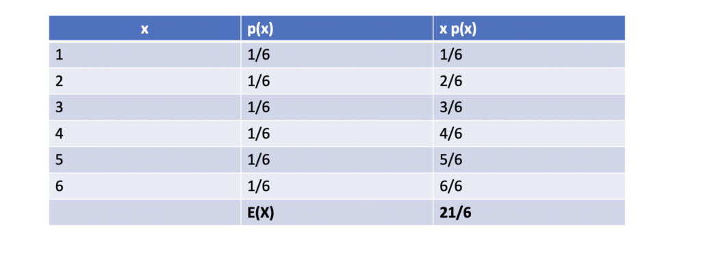
Variance of a Discrete Random Variable
Variance and standard deviation are both measures for how much probabilistic outcomes deviate from the expected value. The variance of a random variable X equals the expected value of the square of X minus the expected value of X squared.
Var(X) = E[(X - E[X])^2]
If you expand the squared expression in brackets, you’ll realize that this is equivalent to the mean of the square of X minus the square of the mean of X.
Var(X) = E[X^2] - E[X]^2
The standard deviation usually denoted as sigma is simply the square root of the variance.
\sigma = \sqrt{Var(X)}Let’s dive right into an example using discrete variables to make this more accessible.
We’ve established that the expected value of a fair dice throw equals 3.5. We simply have to square this
E[X]^2 = 12.25
To obtain the expected value of the square of X, we have to add all the possible squared values that X can assume multiplied by their respective probabilities.
E(X^2) = \frac{1}{6}1^2 + \frac{1}{6}2^2 +\frac{1}{6}3^2 +\frac{1}{6}4^2 + \frac{1}{6}5^2 + \frac{1}{6}6^2 = 15.17Now we can calculate the variance.
Var(X) = E[X^2] - E[X]^2 = 15.17 - 12.25 = 2.92
Sthe standard deviation can now easily be calculated.
\sigma = \sqrt{2.92} = 1.71Often the variance of a discrete random variable is expressed in terms of its concrete values x = {x1,x2,x3,…xn} rather than the random variable X.
Var(X) = \sum_{i=1}^n p(x)_i (x_i - \mu)^2Note that the mean or expected value is usually expressed using the greek letter μ.
The standard deviation can accordingly expressed like this.
\sigma = \sqrt{ \sum_{i=1}^n p(x)_i (x_i - \mu)^2}Expected Value of a Continuous Random Variable
When dealing with continuous random variables, the logic is the same as with discrete random variables. But instead of summing over the possible values x that the random variable X can assume, you take the integral over the interval [a,b] for which you would like to evaluate the probability.
E(X) = \int_a^b xp(x)dx
Assume the outcome of our random variable can be modeled using the following probability density function p(x).
p(x) =\begin{cases}
          \frac{3}{8}(6x - x^2) & 0\leq x\leq 1 \\
          0 & otherwise

       \end{cases}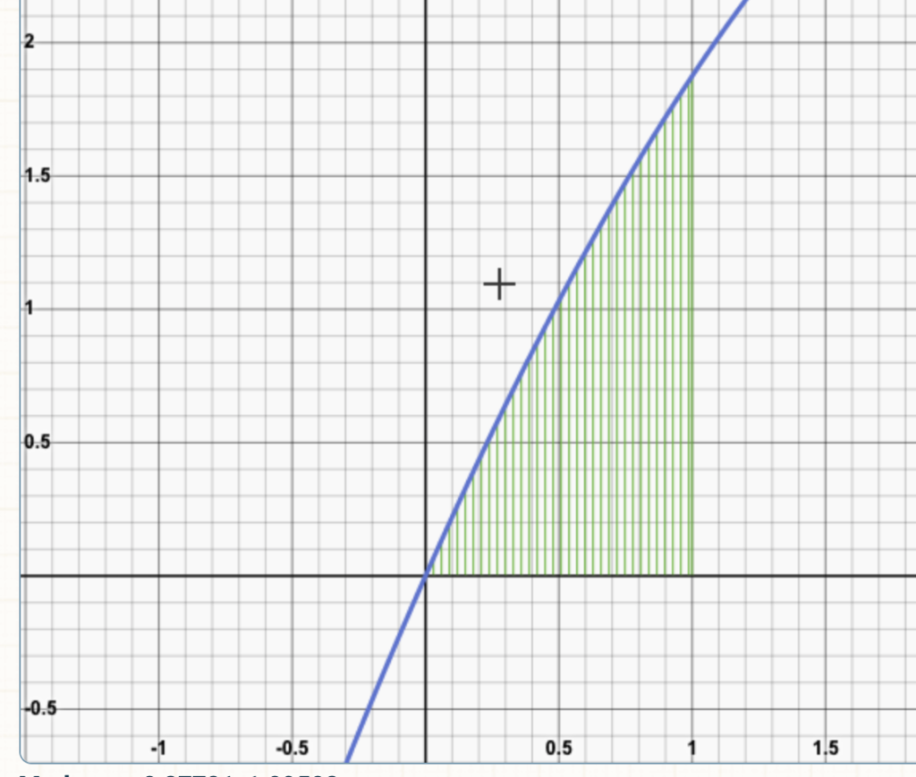
Graph generated with https://www.integral-calculator.com/
First, we plug this into our formula for the expected value:
E(x) = \mu = \int_0^1 x \frac{3}{8}(6x - x^2) dx= \int_0^1 \frac{18}{8} x^2 - \frac{3}{8}x^3Second, we evaluate the integral:
= [ \frac{18}{24} x^3 - \frac{3}{32} x^4 ]_0^2Third, we plug 1 and 0 into the resulting expression:
1 \rightarrow \frac{18}{24} 1^3 - \frac{3}{32} 1^4= 0.65
0 \rightarrow \frac{18}{24} 0^3 - \frac{3}{32} 0^4= 0
Finally, we can evaluate the expression for the interval and thus obtain our expected value.
E(x) = \mu = 0.65 - 0 = 0.65
Variance of a Continuous Random Variable
When using continuous random variables, we have to replace the summation with an integration.
Our variance is calculated as follows.
Var(X) = \int_{-\infty}^{\infty} x^2p(x)dx - \mu^2As in the discrete case, we can also express the variance in terms of the random variable X.
Var(X) = E[X^2] - E[X]^2
Let’s continue with the same function p(x) that we already used for the expected value. Since the function evaluates to zero everywhere except for the interval [0,1], we only need to evaluate the variance for that interval.
We already calculated the expected value (μ = 0.65).
E[x] = \mu = 0.65
So we really just need to evaluate the following expression.
E[X^2] = \int_{0}^{1} x^2p(x)dx = \int_0^1 x^2 \frac{3}{8}(6x - x^2) dx = 0.49This expression is very similar to the calculation we’ve performed for the expected value. The only difference is that the first x is squared. Accordingly, I didn’t list all the steps again.
Now, the variance is just.
Var(X) = E[X^2] - E[X]^2 = 0.49 - 0.65^2 = 0.0675
As with discrete random variables the standard deviation is simply the square root of the variance.
\sigma = \sqrt{Var(X)} = 0.26This post is part of a series on statistics for machine learning and data science. To read other posts in this series, go to the index.


