How do Neural Networks Learn

In this post, we develop an understanding of how neural networks learn new information.

Neural networks learn by propagating information through one or more layers of neurons. Each neuron processes information using a non-linear activation function. Outputs are gradually nudged towards the expected outcome by combining input information with a set of weights that are iteratively adjusted through a process called backpropagation.

The combination of many layers of neurons performing nonlinear data transformations allows the network to learn complex nonlinear relationships in the input data.

Neural Networks as Function Approximation Algorithms

Neural networks can be regarded as algorithms that approximate a mathematical function f*(x). Given a set of training data x and the corresponding output y, we hypothesize that some function exists that takes x as input and produces y.

f^\ast(x) = y

The basic idea of a neural network (and supervised machine learning in general) is to let the algorithm find an approximation to that function through training.
In deep learning, neural networks usually consist of multiple layers. We can treat each layer as a separate function that applies some transformation to the data. Depending on the number of layers, our neural network attempts to approximate f*(x) through a series of nested functions.

f^1(f^2(f^3(x))) = f^\ast(x) = y

Understanding a Neural Network Step By Step

How does a neural network construct a function that allows it to determine whether an image contains a cat or to represent an English sentence in French?

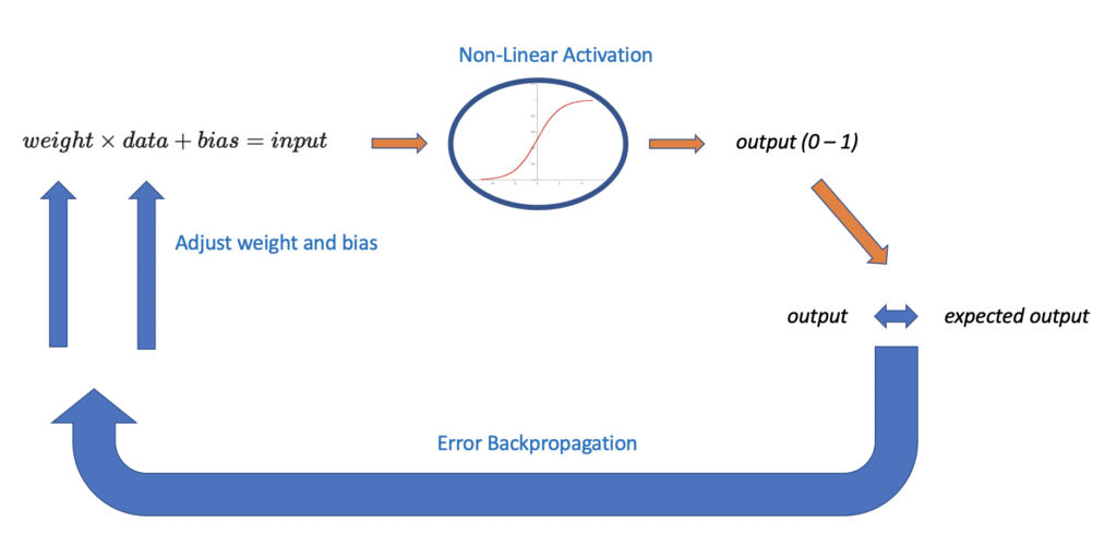
To understand how this works, let’s have a high-level look at a single neuron processing a single data point.
First, we multiply our data with a randomly chosen weight and add a randomly chosen bias. The result is our input to the neuron. We need the bias and the weight so that we can influence the result produced by the neuron. This is crucial to learning.

weight \times data + bias = input

Next, we send the result through a neuron, which represents a non-linear activation function. The activation function transforms our input into a value in a specific range (usually between 0 and 1).

Now, we compare the output produced by the nonlinear activation function to the expected output. We measure the difference using a cost function. The larger the discrepancy between the produced and the expected output, the larger the imposed cost.

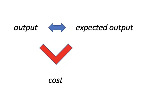
Finally, we send the information on how far off the produced result is from the expected back to the beginning. We use this information to slightly adjust the weight and the bias. Through a process called backpropagation, which is based on the chain rule of differentiation, we can gradually adjust the weights and biases in the desired direction. Then we repeat the process with the updated weights and biases until our produced output is reasonably close to the expected output.

In a deep neural network, you have thousands of these neurons stacked in multiple layers. How do these neurons interact to produce an output? And why do we need a non-linear activation function?

Now that we have a high-level understanding of the basic principles by which a neural network learns, we can dive into the details and address these questions.

Neural Network as Logistic Regression

If you are familiar with logistic regression, you are in a very good position to understand neural networks. A logistic regression model is basically a neural network with only one layer and one neuron.

We still multiply our input data with a weight and add a bias. From here on, we will adopt the convention of calling the input data x, the weight w, and the bias b. Together they produce the output z. x

z = wx + b

Since we are dealing with vectors of values rather than single values, w, x, b, and z all become vectors or matrices. For reasons that will become clear when we deal with neural networks, we structure our weight vector so that its transpose will be multiplied by x.

z = w^Tx + b

Next, we send the output z through a sigmoid activation function, which is a non-linear function that transforms an input to a value between 0 and 1.

\sigma(z) = \frac{1}{1+e^{-z}}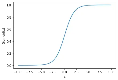

As you can see on the graph, very large values result in an output close to 1, while small values result in an output close to 0.
Although the analogy is imperfect and neural networks are only loosely inspired by the brain, you can think of it as a biological brain cell. Once a brain cell receives enough stimulus, it will fire off an electric signal. Here, z is like the stimulus that is supplied to the cell, while the output produced by the cell is like the signal that is further transmitted. Therefore, the sigmoid function is called an activation function. It decides whether the cell will activate and fire off a signal or not.

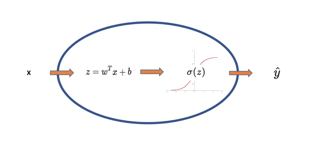
The neuron accepts the data as input, multiplies it with a weight and adds a bias, and finally transforms it to a value between 0 and 1 by sending it through a sigmoid activation function. The resulting signal y hat is compared to the expected outcome y.

With that knowledge in place, we can move on to constructing a neural network.
If you want to learn more about logistic regression and how the whole learning process works, check out my post on logistic regression.

Forward Propagation in a Neural Network Step by Step

In a neural network, you have several of the previously described neurons stacked on top of each other in layers. A network may consist of several layers.

For the sake of simplicity, let’s look at a very simple neural network with two layers and three neurons in the first layer.

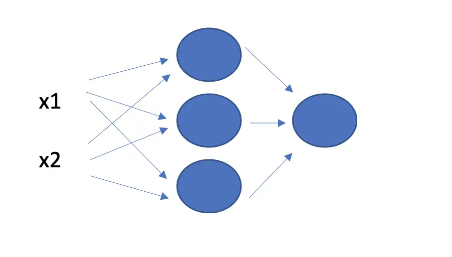
Each observation in the dataset is sent through all the neurons in the first layer. This means each neuron needs to provide a vector of weights that equals the number of observations in length. Otherwise, we wouldn’t be able to multiply the weights with the input.

x =
 \begin{bmatrix}
x_1 \\
x_2
 \end{bmatrix} 

w = 
 \begin{bmatrix}
w_1 \\
w_2
 \end{bmatrix} 

But we don’t just have one neuron but three. We can stack all of them in a matrix W.

W = 
 \begin{bmatrix}
w_1^1 & w_1^2 & w_1^3 \\
w_2^1 & w_2^2 & w_2^3
 \end{bmatrix} 

The superscript represents the neuron the weight belongs to.
I’m violating mathematical convention here because the superscript usually represents a power operation. But for the rest of this post, we will use it to note the neuron in a given layer.

To perform the multiplication of the input data with the weights across all observations and neurons in the layer, we transpose the matrix.

W^Tx =   \begin{bmatrix}
w_1^1 & w_2^1 \\ w_1^2 & w_2^2 \\ w_1^3 & w_2^3 \\
 \end{bmatrix} 
 \begin{bmatrix}
x_1 \\
x_2
 \end{bmatrix} 
=
 \begin{bmatrix}
w_1^1x_1  + w^1_2x_2\\
w_1^2x_1  + w^2_2x_2\\
w_1^3x_1  + w^3_2x_2\\
 \end{bmatrix} 

If you don’t know how matrix multiplication works, check out my post on the topic.

Lastly, we can also add the bias term, which gives us the output z as a vector with 3 entries.

W^Tx + b =   \begin{bmatrix}
w_1^1 & w_2^1 \\ w_1^2 & w_2^2 \\ w_1^3 & w_2^3 \\
 \end{bmatrix} 
 \begin{bmatrix}
x_1 \\
x_2
 \end{bmatrix} 
+
 \begin{bmatrix}
b^1 \\
b^2 \\
b^3
 \end{bmatrix} 
=
 \begin{bmatrix}
(w_1^1x_1  + w^1_2x_2) + b^1\\
(w_1^2x_1  + w^2_2x_2) + b^2\\
(w_1^3x_1  + w^3_2x_2) + b^3\\
 \end{bmatrix} 
 =
 \begin{bmatrix}
z^1\\
z^2\\
z^3\\
 \end{bmatrix} 
= 
z

So now we have a z value for each neuron. From logistic regression, we know that we need to send each z value through a sigmoid function to obtain the predicted value y hat. But in this case, we have not yet arrived at y hat because there is still another layer. Instead, we use an intermediate value a.

a =  \begin{bmatrix}
a_1\\
a_2\\
a_3\\
 \end{bmatrix} 
=  \begin{bmatrix}
\sigma(z^1)\\
\sigma(z^2)\\
\sigma(z^3)\\
 \end{bmatrix} 

Now that we have arrived at a, we no longer need to keep track of neurons and observations in the input data, so we simply denote a as a vector with three entries marked by a subscript and dispense with the superscript notation.

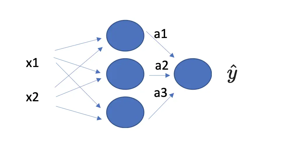
To represent the operations mathematically so far, we relied on the subscript to represent the observation in the dataset and the superscript to represent the neuron in the current layer.

But since we have more than two layers, we have to introduce a third dimension to represent the layer. We denote the layer in square brackets as follows.

a^{[1]}  =  \begin{bmatrix}
a_1^{[1]} \\
a_2^{[1]}\\
a_3^{[1]}\\
 \end{bmatrix} 

This means the vector a represents the intermediate output of the first layer.

To arrive at our final prediction y hat, we need to pass the vector through the same procedure for the next layer, which only consists of one neuron:

• mutiply a with a vector of weights associated with the neuron
• add a bias associated with the neuron
• pass the resulting term through a non-linear activation function

With the layer notation in place, we can succinctly describe these operations mathematically as follows:

z^{[2]} = W^{[2]t} a^{[1]} + b^{[2]}

\hat y = \sigma(z^{[2]})

I’ve adopted this convention from Andrew Ng’s Deep Learning course on Coursera.

We can equally express the full neural network operation from start to finish.

First, we send the input data through the first layer, multiplying with the weights, adding a bias, and passing the whole expression through the sigmoid function.

z^{[1]} = W^{[1]t} x + b^{[1]}

a^{[1]} = \sigma({z^{[1]}})

Then we pass the result from the first laxer through the second layer, which gives us the output y hat.

 z^{[2]} = W^{[2]t} a^{[1]} + b^{[2]}

\hat y = \sigma(z^{[2]})

Understanding Matrix Multiplication in Neural Network Forward Propagation

In this example, we’ve used a 1-dimensional vector for x rather than a 2-dimensional matrix. As a consequence, the math was a bit easier to follow. But a real training dataset will consist of many training examples and multiple features. Accordingly, the input becomes higher-dimensional. For example, if your input consists of RGB images, then you will have 4 dimensions representing the number of images, the pixels on the x-axis, the pixels on the y-axis, and the color channels.

Your input layer will always have the same dimension as the input dataset. Your weight matrix needs to have a dimensionality that allows you to multiply it with the input data and to pass it through the next layer.

In practice, this means your weight matrix’s number of rows has the be equivalent to the number of units in the next layer, while its number of columns needs to be equivalent to the number of rows in the input dataset.

While modern deep learning frameworks like Tensorflow will take care of the internal calculation, you still need to be aware of how the calculations affect the dimensionality of your data as it passes through the layers.

A Note on Activation Functions

In the previous sections, I’ve referred to non-linear activation functions. But why do we actually need non-linear functions?
If you apply a linear function, your data will always be some multiple of the original data. In a machine learning context, this means you won’t be able to represent non-linear decision boundaries. Our goal in training a neural network is to model a function that represents a non-linear decision boundary.
The combination of multiple non-linear activation functions allows a neural network to learn extremely complex non-linear relationships in data.

In previous sections, we’ve always used the sigmoid function as an example for a non-linear activation function. In fact, there are several more functions, such as the hyperbolic tangent, the rectified linear unit, and the leaky rectified linear unit. In most cases, these functions are a better fit for neural network activation than the sigmoid function. I will introduce these functions and discuss their merits in a future post.

The Cost Function

Once you’ve sent your data through the neural network in the forward pass and calculated the output y hat, you need to measure how far the predictions diverge from the expected output y. To force the neural network to improve its predictions, you impose a cost on it that is a function of the difference between the predicted output y hat and the expected output y.
During neural network training, this is done using a cost function. Since you want to adjust the weights and the biases to improve the learning outcome, the cost is defined as a function of the weights and the biases.

J(W, b) 

The cost is calculated as the total difference between all predicted and expected outcomes. The difference between one predicted and one expected outcome is known as the loss.

L(\hat y, y)

To get to the cost, we need to calculate the average of all losses in our dataset.

J(W, b) = \frac{1}{n} \sum_{i=1}^{n} L(\hat y_i, y_i)

But how do you actually measure the difference between predicted and expected outcomes?
In neural networks for binary classification, a common measure for the loss is the cross-entropy which is also known as the negative log-likelihood.

L = -(y \; log(\hat y) + (1-y)log(1-\hat y))

There are several different loss functions and which one you choose depends on the type of machine learning problem you are facing. Here is a great overview.

Backpropagation with Gradient Descent

The ultimate step in neural network learning is backpropagation. I will discuss backpropagation on a conceptual level without going into the mathematical details since it involves advanced calculus. You don’t need to understand these details when building deep learning systems in practice. Frameworks like Tensorflow will take care of it for you.

The goal of backpropagation is to adjust the parameters (weights and biases) of your neural network to minimize the cost function. This means you need to communicate the cost that you calculate at the end of forward propagation back to the very beginning so you can adjust the original weights and biases.

Using derivatives from calculus, we can calculate how the change in one variable affects a change in another one.
For example, to figure out how a change in a parameter w affects the cost, we can take the derivative of the cost with respect to w (the procedure is similar for the weights).

\frac{dJ}{dw}

This expression is known as the gradient. The weight vector w can be visualized as a vector in a multidimensional space. The gradient is a vector that points in the direction of the steepest slope. In other words, it tells us in what direction we have to adjust the values for w in order to minimize the cost J. To learn more about this procedure, check out my post on gradient descent.

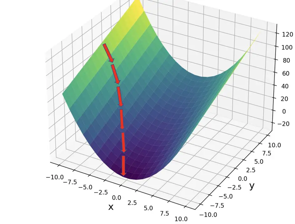
With gradient descent, we repeatedly calculate the gradient and subtract it from the weight vector. Then we move through forward propagation with the adjusted weights, which should result in a reduced cost. This process is repeated until we reach a small enough cost.

w_{new} = w - l \frac{dJ}{dw}

The term l is the learning rate that determines the speed with which the neural network learns. It is a very small term since subtracting the full gradient will lead the network to overshoot.

The original weight and bias that we want to adjust are only related to the cost through a series of intermediate transformations defined by the layers in the neural network. For example, the 2-layer neural network we defined above w is transformed through the following equations defining forward propagation followed by the cost function.

z^{[1]} = W^{[1]t} x + b^{[1]}

a^{[1]} = \sigma({z^{[1]}})

 z^{[2]} = W^{[2]t} a^{[1]} + b^{[2]}

\hat y = \sigma(z^{[2]})

J = \frac{1}{n} \sum_{i=1}^{n} L(\hat y, y)

We have to backpropagate the error captured by the cost function through all the intermediate steps to correctly adjust the initial weights and biases. This is where the chain rule from calculus comes into play. The chain rule allows us to take the derivative of the cost with respect to the original W by chaining derivatives of the intermediate values together.

\frac{dJ}{dW^{[1]}} = \frac{dJ}{d\hat y} \frac{d\hat y}{ dz^{[2]} } \frac{ dz^{[2]} }{da^{[1]}} \frac{da^{[1]}}{ dz^{[1]} } \frac{ dz^{[1]} }{dW^{[1]}}

The chain rule is at the heart of backpropagation. Now, you have a conceptual understanding of how a neural network learns information.

This article is part of a blog post series on the foundations of deep learning. For the full series, go to the index.