An Introduction to Residual Skip Connections and ResNets

In this post, we will develop a thorough understanding of skip connections and how they help in the training of deep neural networks. Furthermore, we will have a look at ResNet50, a popular architecture based on skip connections.

What are Residual Skip Connections?

In a nutshell, skip connections are connections in deep neural networks that feed the output of a particular layer to later layers in the network that are not directly adjacent to the layer from which the output originated.

In the following sections, we are going to look at skip connections in detail and understand how they mitigate the problem of vanishing gradients and degrading accuracy that often accompany very deep neural network architectures.

Why Do We Need Skip Connections?

As researchers designed neural networks with more and more layers, the problem of vanishing and exploding gradients became increasingly prominent.
Vanishing and exploding gradients are more problematic in deep networks because, during backpropagation, each additional layer adds values to the multiplication we need to perform to obtain the gradient.
If you don’t know why this is the case, check out my post on vanishing and exploding gradients.

If you multiply several values that are smaller than 1 together, the result will shrink exponentially with every term you add to the multiplication.
If you multiply several terms that are larger than 1 together, the result will grow exponentially with every term you add to the multiplication. The more layers we have, the more multiplications we have to perform.

Furthermore, it has been empirically verified that the performance of very deep neural networks with traditional architectures tends to degrade, and accuracy saturates as the network converges.

To alleviate these problems, a skip connection bypasses one or more layers and their associated operations.

How Skip Connections Work

If the output of one of the earlier layers is x_0, a traditional neural network would perform the following operations in the next layers.

z_1 = w_1 x_0 + b_1

x_1 =ReLU(z1)

z_2 = w_2 x_1 + b_2

x_2 = ReLU(z_2)

With a skip connection, you still perform these operations, but in addition, x_0 also bypasses them and rejoins the output before the second activation function through simple addition.

x_2 = ReLU(z_2 + x_0)

The ReLU activation function outputs the input directly if it is positive. Thus, If z_2 were equal to 0 and we only passed (positive) x_0 through the ReLU activation, the output would be as follows.

x_2 = ReLU(0 + x_0) = x_0

In other words, the skip connection essentially calculates the identity function of x_0. This fact will come in handy in the next sections when we try to understand why residual networks work so well.

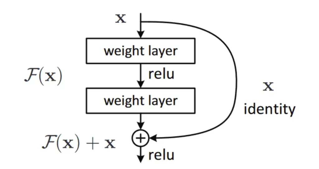
Taken together, these operations form a residual block.

How do Skip Connections Address Vanishing Gradients and Degrading Accuracy?

Let’s summarize the intermediate calculations in the residual block without skip connections as a function.

F(x)

Since we don’t need the intermediate x value anymore, x is equivalent to x_0 in the following explanations.

When we introduce a skip connection that lets x_0 bypass all calculations in F(x). We express this new operation as H(x). Since x is added to the output of F(x), H(x) looks like this:

H(x) = F(x) + x

During the intermediate calculations, F(x) may become very small or otherwise change in a way that degrades the ability of the neural network to learn a complex mapping. In practice, the likelihood that this will happen increases as you add more layers to a network. By adding x, you are adding the identity mapping of the input to F(x). This gives the network a kind of baseline for the function it has to learn. Remember that the basic goal of a neural network is to find a mapping.

x \rightarrow  y

In the worst case, when using a skip connection, the network could fall back to using the identity mapping.

x \rightarrow x

In deep networks, this gives the model the ability to ignore the mapping of specific layers. Imagine you built a network with 300 layers, and it turned out that 50 layers are just fine to learn your problem; skip connections and residual blocks would allow your network to bypass the remaining 250 layers.

During backpropagation, we differentiate the loss function with respect to the weights. To get to the weights in earlier layers, we have to differentiate through all the intermediate functions represented in the previous layers. Let’s imagine for a moment that the last activation function in the residual block produces the final output and that we calculate the cost J right afterward.
To propagate the gradient back to the layers before the residual block, we, therefore, need to calculate the gradient of the cost with respect to x.

\frac{\partial J}{\partial x} 

Using the chain rule, the full operation with all the intermediate steps to be performed without the skip connection looks like this:

\frac{\partial J}{\partial x_0}  =
\frac{\partial J}{\partial x_2}  \frac{\partial x_2}{\partial z_2} \frac{\partial z_2}{\partial x_1}  \frac{\partial x_1}{\partial z_1}  \frac{\partial z_1}{\partial x_0} 

This is a long series of multiplications that, as mentioned above, makes neural networks susceptible to vanishing and exploding gradients.

If we replace the intermediate calculations by F(x), the gradient calculation now becomes:

\frac{\partial J}{\partial x}  = \frac{\partial J}{\partial F(x)}  \frac{\partial F(x)}{\partial x} 

When adding the skip connections, we introduced the additional function H(x) = F(x) + x. To calculate the gradient of the cost function in a network with skip connections, we now need to differentiate through H(x).

\frac{\partial J}{\partial x}  = \frac{\partial J}{\partial H(x)}  \frac{\partial H(x)}{\partial x} 

The derivative of x with respect to x is equal to 1. Thus, substituting F(x) + x for H(x) gives us the following expression:

\frac{\partial J}{\partial x}  =  \frac{\partial J}{\partial H(x)}  \left( \frac{\partial F(x)}{\partial x}  + 1 \right) = \frac{\partial J}{\partial H(x)}  \frac{\partial F(x)}{\partial x} + \frac{\partial J}{\partial H(x)}

Even if the gradient of F(x) becomes vanishingly small due to the many multiplications performed when backpropagating through all the layers, we still have the direct gradient of the cost function with respect to H(x).
That way, the network can also skip some of the gradient calculations during backpropagation and prevent the gradient from vanishing or exploding.

What Skip Connections Learn

Conceptually, the layers in a convolutional neural network learn features in increasing levels of abstraction. Skip connections allow a deep neural network to pass lower-level semantic information unchanged to the latter layers of the neural network. This helps preserve information that would have been abstracted away if it had been passed through too many layers.

The ResNet50 Architecture

The primary architectures that build on skip connections are ResNets and DenseNets. After AlexNet, ResNets constituted the next big breakthrough in deep learning for computer vision, winning the imagenet classification challenge in 2015. As expected, the main advantage of ResNets was that they enabled the construction of much deeper neural networks without running into exploding and vanishing gradients or degradation of accuracy.

The first ResNet architectures ranged from 18 layers to 152 layers. Nowadays, some researchers rely on skip connections to construct networks with more than 1000 layers.

For illustration, let’s have a look at ResNet50, a common ResNet architecture with a total of 50 layers.

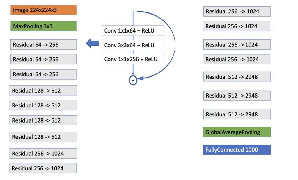
The architecture takes a 224x224x3 image as input, followed by a MaxPooling layer with a 3×3 filter. Then it has 16 residual blocks. Each residual block consists of 3 convolutional layers that transform the dimensionality of the data, as indicated in the illustration. The residual blocks form 4 groups. Within a group, the residual blocks have similar layers. For example, in the first group, we have three residual blocks that each consist of 3 convolutional layers that perform the following convolutions.

• 1x1x65
• 3x3x64
• 1x1x256

In the second group, we have 4 residual blocks with 3 convolutional layers that perform the following convolutions:

• 1x1x128
• 3x3x128
• 1x1x512

The third group consists of 6 residual blocks with 3 convolutional layers:

• 1x1x256
• 3x3x256
• 1x1x1024

The last group has 3 blocks, each of which has layers performing the following convolutions:

• 1x1x512
• 3x3x512
• 1x1x2948

Lastly, the architecture performs global average pooling before feeding the feature map to a fully connected layer that distinguishes between the 1000 images used in the ImageNet database.

This article is part of a blog post series on deep learning for computer vision. For the full series, go to the index.