Deep Learning Architectures for Image Classification: LeNet vs Alexnet vs VGG

In this post, we will develop a foundational understanding of deep learning for image classification. Then we will look at the classic neural network architectures that have been used for image processing.

Deep Learning for Image Classification

Image classification in deep learning refers to the process of getting a deep neural network to determine the class of an image on the basis of a set of predefined classes. Usually, this requires the network to detect the presence of certain objects or backgrounds without the need to locate these objects within the image.

For example, a neural network trained to classify images by the type of pet they contain would be able to detect the presence of a cat in an image and distinguish a cat from other pets.

Why Do We Use Convolutional Neural Networks in Image Processing?

Early image processing techniques relied on understanding the raw pixels. The fundamental problem with this approach is that the same type of object can vary significantly across images. For example, two pictures of cars might be taken in by cars of different colors and at different angles. It is extremely difficult for a method that relies on understanding single pixels to generalize across the large variety inherent in pictures of objects.
Furthermore, it is extremely inefficient to try to understand single pixels without the surrounding context.
This inefficiency and lack of context are some of the main reasons why traditional fully connected networks are inappropriate for most image classification tasks.
To feed an image to a fully connected network, you would have to stack all the pixels in an image in one column.

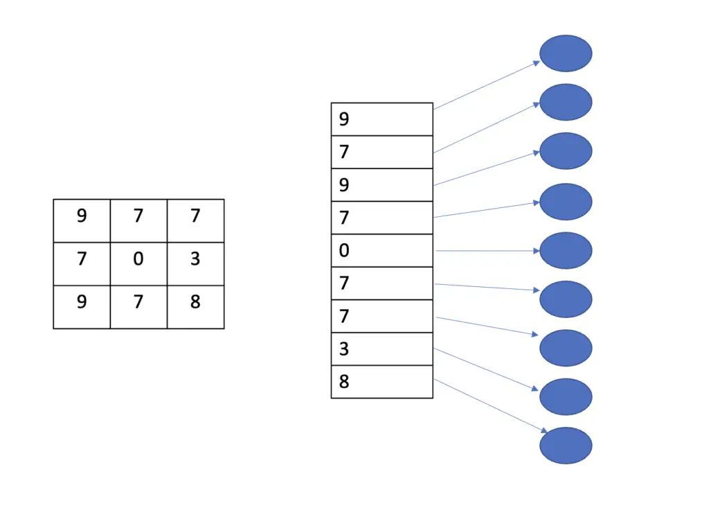
Individual pixels are taken out of the context of the surrounding pixels and are fed individually to a neuron that will perform a classification. If you had a grayscale image of 512×512 pixels, you would need 512×512 = 262144 neurons just in your first layer to classify every pixel. Since you connect each pixel to each pixel in the next layer, your number of parameters will explode into millions or billions just for a simple image classification model.
This approach works for simple tasks like distinguishing between 10 handwritten digits. But for anything more complex, you want a method that can incorporate the context, and that can also reuse information across pixels.

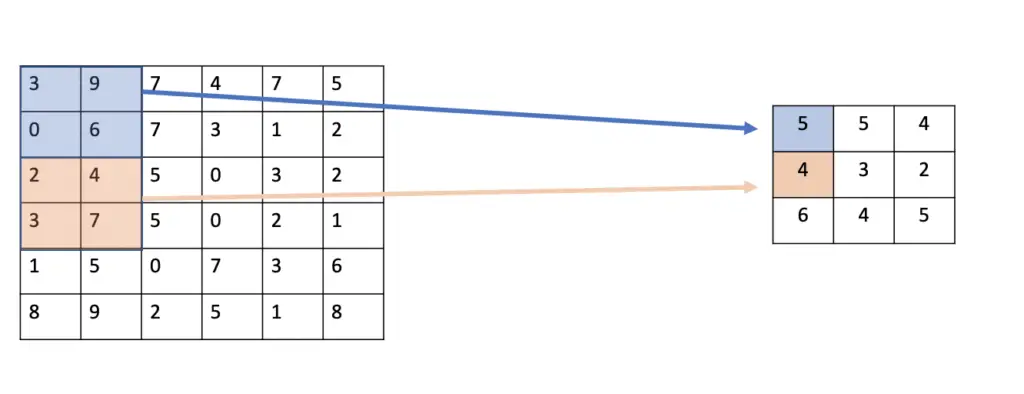
Instead of classifying individual pixels directly, convolutional layers slide filters over the image. These filters can understand pixels in the context of the other surrounding pixels to extract features such as edges. The network then only learns to detect the presence of the feature. Non-linear activation functions are used to make detection decisions resulting in a feature map that stores information about the presence of the feature in the image and its correspondence to the filter.

This process entails two main advantages. Firstly, filters are not limited to one group of pixels. They can be reused across the entire image to detect the presence of the same feature in other areas of the image. The result is that parameters are shared and reused.
Secondly, the output of a filter only connects to one field in the parameter map of the next layer as opposed to connecting every node in one layer to every node in the next layer. As a consequence, the number of parameters is dramatically reduced, resulting in sparse connections.

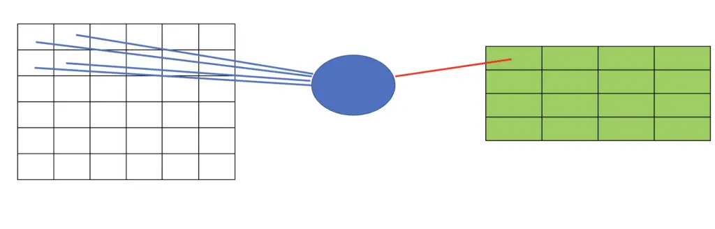
Note that convolutional neural networks do have fully connected layers. You usually find them in the latter part of the network because they ultimately lead into the final classification layer that produces the decision of what class the image belongs to. By the time you reach the later layers, the feature maps produced by the convolutional layers will have reduced the original image to a limited set of features so that a fully connected layer can reasonably be applied to distinguish between those features and decide whether they constitute the desired object.

LeNet-5

LeNet is one of the earliest convolutional neural networks that was trained in 1990 to identify handwritten digits in the MNIST dataset.
It only consists of 5 layers (counting a pooling and a convolutional layer as one layer) and has been trained to classify grayscale images of size 32×32. Due to the comparatively small number of parameters and simple architecture, it is a great starting point for building an intuitive understanding of convolutional neural networks.
Here is an illustration of the network architecture from the original paper.

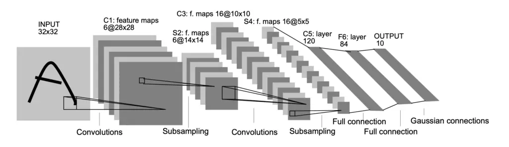
Let’s briefly walk through the architecture.

• We use a 32x32x1 image as input. Since the images are grayscale, we only have one channel. The first convolutional layer applies 6 5×5 filters. As a result of sliding the 6 5×5 filters over the input image, we end up with a feature map of 28x28x6. If you don’t understand why this is th case, I recommend reading my article on convolutional filters first. The convolutional layer uses a tanh activation function.
  
• After the first convolutional layer we have an average pooling layer with a filter size of 2×2 and a stride of 2. The resulting feature map has dimensions 14x14x6. Again, if you couldn’t follow that reasoning, check out my article on pooling.
• The network has another convolutional layer that applies 16 5×5 filters as well as a tanh activation function resulting in an output map of 10x10x16.
• The convolutional layer is followed by another pooling layer with a filter size of 2×2 and a stride of 2 producing a feature map of 5x5x16
• We have a final convolutional layer with 120 filters of size 5×5 and a tanh activation resulting in a feature map of 1x1x120, which connect neatly to a fully connected layer of 120 neurons.
• Next, we have another fully connected feature map of 84 neurons. The fully connected layers both have tanh activation functions.
• Finally, we have the output layer that consists of 10 neurons and a softmax activation function since we have a multiclass classification problem with 10 different classes (one for each digit).
  

As you can see, the network gradually reduces the size of the original input image by repeatedly applying a similar series of operations:

• Convolution with a 5×5 filter
• Tanh activation
• Average pooling with a 2×2 filter

These operations result in a series of feature maps until we end up with a 1x1x120 map. This allows us to make the transition to fully connected layers while the rest of the neural network operates like a traditional fully connected network.
Note that the convention of using tanh as an activation function between layers and applying average pooling is not common in modern convolutional architectures. Instead, practitioners tend to use ReLU and max pooling.

AlexNet

AlexNet initiated the deep learning revolution in computer vision by pulverizing the competition in a 2012 computer vision contest. The network is significantly larger than LeNet, which partly explains why there was a gap of more than 20 years between LeNet and AlexNet. In the 1990s, computational power was so limited that training large-scale neural networks wasn’t feasible.
The number of classes AlexNet was able to handle compared to LeNet also increased significantly from a mere 10 to 1000. Consequently, it was also trained on a much larger dataset comprising millions of images.

AlexNet can process full RGB images (with three color channels) at a total size of 227x227x3.

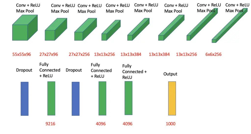
AlexNet relies on similar architectural principles as LeNet. It uses 5 pairs of convolutional layers and pooling layers to gradually reduce the size of the feature maps along the x and y axes while increasing the filter dimension. Ultimately, the last feature map connects to a series of 3 fully connected layers resulting in an output layer that distinguishes between 1000 classes using a softmax activation.

Compared to LeNet, the AlexNet architecture also featured some innovations:

• ReLU activation function which accelerated learning signifcantly compared to tanh
• Applying max pooling instead of average pooling
• Overlapping pooling filters to reduce the size of the network which also resulted in a decrease in error
• Dropout layers after the last pooling layer and the first fully connected layer to improve generalization and reduce overfitting.

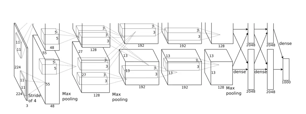
The full feature map transformation across the layers looks as follows.

For training, the architecture was split between two GPUs, with half of the layers being trained on one GPU and the other half on the other GPU.

While AlexNet marked a quantum leap in the development of convolutional neural networks, it also suffered from drawbacks.

Firstly, the network had approx. 60 million parameters which make it not only large but also extremely prone to overfitting.
Compared to modern neural network architectures, AlexNet was still relatively shallow. Modern networks achieve great performance through increasing depth (which comes with its own drawbacks, such as exploding and vanishing gradients).

Alexnet applied unusually larger convolutional filters of up to 11×11 pixels. Most recent architectures tend to use smaller filter sizes such as 3×3 since most of the useful features are found in clusters of local pixels.

VGG 16 and VGG 19

VGG 16 marked the next large advance in the construction of neural network architectures for image processing. Arriving in 2014, it achieved a 92.7% test accuracy in the same contest that AlexNet had won 2 years prior.
VGG 16 is based on AlexNet, but it made some critical changes. Most notable is the increase in depth to 16 layers and the simplification of the hyperparameter tuning process by using only 3×3 filters.

Why Do Deep Neural Networks Work Better?

While there is no definitive answer to this question, several theories have been proposed as to why depth improves the performance of neural networks.

The first explanation relies on the fact that neural networks attempt to model highly complex real-world phenomena. For example, when trying to recognize an object in an image, a convolutional neural network assumes that there must be some function that explains how the desired object differs from other objects and attempts to learn this function.
Each layer in a neural network represents a linear function followed by a non-linear activation to express non-linearities in the data. The more of these layers you combine, the more complex the relationships that the network can model.

Another argument stipulates that more layers force the network to break down the concepts it learns into more granular features. The more granular the features, the more the network can reuse them for other concepts. Thus, depth may improve generalizability. For example, when training a convolutional neural network to recognize cars, one layer in a relatively deep network may only learn abstract shapes such as circles, while a layer in a relatively shallow network may learn higher-level features that are specific to a car, such as its wheels.

For convolutional neural networks, another idea suggests that increasing depth results in a larger receptive field. Since you are stacking multiple small filters on top of each other where each summarizes the content in the preceding filter, the layers later in the network will have a higher bird-view perspective on the image. If you used a shallow network, the layers would need larger filters to capture the entire image.

How Does the Filter Size Affect the Convolutional Neural Network (CNN)

In practice, most neural network architectures rely on 3×3 or 5×5 filter sizes. Larger filter sizes such as the 11×11 used in AlexNet have fallen out of favor.

Firstly, they result in a larger increase in the parameter space. A filter of size 11×11 adds 11×11 = 121 parameters, whereas a 3×3 filter only adds 9 parameters. Stacking 2 or 3 3×3 filters only results in a total of 18 or 27 parameters which is still much less than 121.

Secondly, each filter comes with a non-linear activation function of the corresponding layer. Stacking multiple filters with non-linear activation functions for each one enables the network to learn more complex relationships than a single larger filter with only one activation function.

VGG 19 Architecture

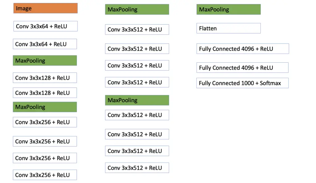
The VGG 19 Network takes a picture of size 224x224x3 as input. The structure of the convolutional layers is the same throughout the network. They all use 3×3 filters and same padding with a stride of 1 to preserve the dimensions of the input.

The image is passed through 2 convolutional layers with 64 3×3 filters followed by a Max Pooling layer. The pattern is repeated another time with 2 convolutional layers with 128 filters each followed by a max-pooling layer.

Then we have 3 blocks with 4 convolutional layers and a max-pooling layer per block. The number of filters equals 128 in the first block and is increased to 512 in the latter two blocks. Finally, we have a layer to flatten the input, followed by 3 fully connected layers. All convolutional and fully connected layers use the ReLU activation function except for the last one which uses the softmax to distinguish between the 1000 classes.

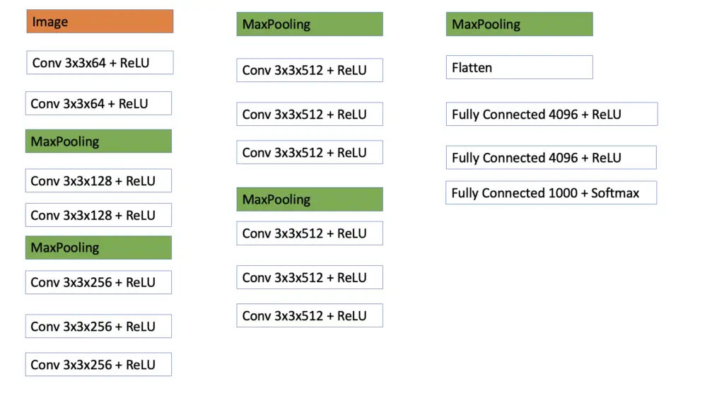
VGG 16 Architecture

The VGG16 Architecture is, in principle, the same as the VGG 19 architecture. The main difference is that the 3rd, 4th, and 5th blocks only have 3 convolutional layers.

This article is part of a blog post series on deep learning for computer vision. For the full series, go to the index.