An Introduction to Convolutional Neural Network Architecture

In this post, we understand the basic building blocks of convolutional neural networks and how they are combined to form powerful neural network architectures for computer vision. We start by looking at convolutional layers, pooling layers, and fully connected. Then, we take a step-by-step walkthrough through a simple CNN architecture.

Understanding Layers in a Convolutional Neural Network

Layers are the basic building block of neural network architectures. Convolutional neural networks primarily rely on three types of layers. These are convolutional layers, pooling layers, and fully connected layers.
Let’s have a look at each of them.

What is a Fully Connected Layer

Fully connected layers are the most elementary layers. They consist of a string of neurons stacked on top of each other.

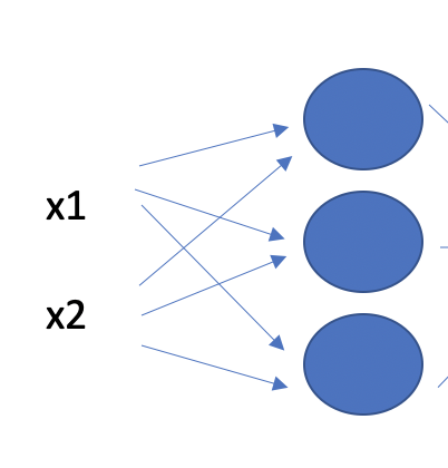
Each neuron takes x as an input, multiplies it with a weight, and adds a bias.

wx + b

The result is sent through a non-linear activation function such as the ReLU to calculate an output that is sent to the next layer.

relu(wx+b)

What is a Convolutional Layer

A convolutional layer is a layer in a neural network that applies filters to detect edges and structures in images. By using multiple convolutional layers in succession, a neural network can detect higher-level objects, people, and even facial expressions.

The main reason for using convolutional layers is their computational efficiency on higher-dimensional inputs such as images. If we wanted to train a fully connected layer to classify images, we would have to roll out the 2D image into a one-dimensional stack of pixels. For example, an image with a dimension of 200×200 would become a stack of 4000 pixels. Our fully connected layer would have to contain 4000 units to learn each pixel value.

In a convolutional layer, we replace the multiplication of x with a weight w with a convolution operation. Instead of w, we use a 2-dimensional filter k that we convolve with our input image x.

For an explanation of how the convolution operation works, check out the post on convolutional filters.

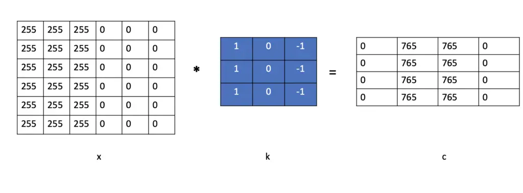
Then, like in a fully connected layer, we add a bias to the result of the convolution c and send the final result through a non-linear activation function such as the ReLU.

a= relu(c+b)

Output Dimensions of a Convolutional Layer

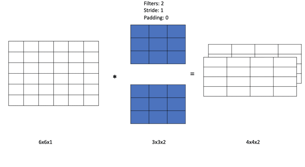
You may have realized that the original image we fed to the convolutional layer had a dimensionality of 6×6, but the output was 4×4. Understanding how the convolution operation changes the dimensions of your input is crucial to getting your convolutional neural networks to work. The change of dimensions in a convolutional layer depends on the size of the filter, the stride, and the padding. The filter changes the image dimensions by a factor of

(m\times m) * (f\times f) = (m-f+1)*(m-f+1)

where m is the image length, and f is the filter length. The stride manipulates the output size by changing the step size with which we move the filter over the image, while the padding enables us to add a border around the image to prevent shrinkage due to the filter size. To understand exactly how these operations influence the size of the output, check out this post on padding, stride, and kernel sizes.

Furthermore, convolutional layers usually slide multiple filters over the image. As a result, their output will contain three dimensions even if you only feed it a 2-d image.

What is a Pooling Layer

A pooling layer is a layer in a convolutional neural network that abstracts the features extracted by a convolutional layer and helps make the features invariant to translations. To achieve this, it applies the pooling operation on the output produced by the convolutional layer.

To learn more about the pooling operation, check out this post on pooling.

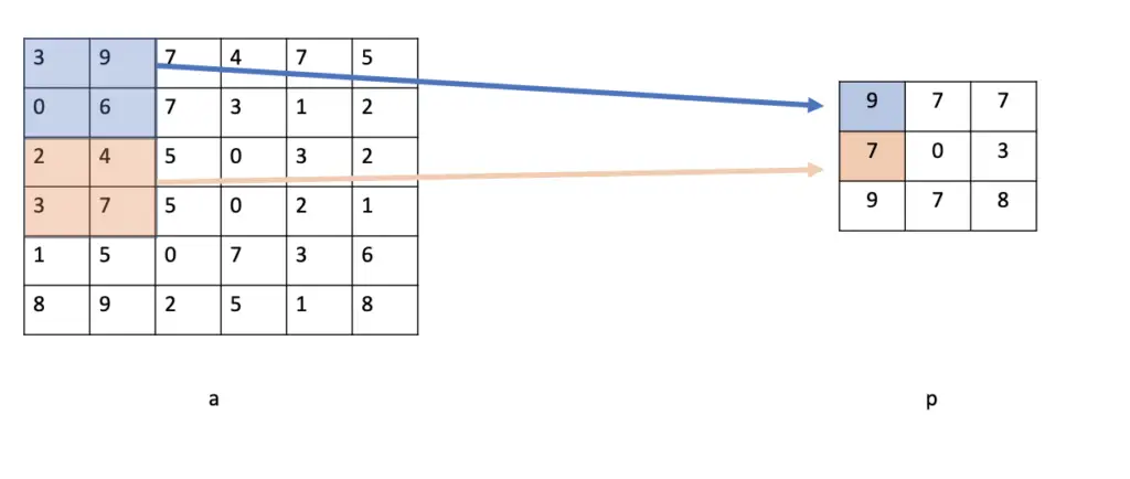
The pooling layer is fairly simple. It only slides a filter over the output of the convolutional layer, selects the highest pixel value under the filter (provided we use max-pooling), and produces the output in a multidimensional map p.

Output Dimensions of a Pooling Layer

The pooling layer also shrinks the output depending on the size of the pooling filter and the stride or step size with which we move the filter. Commonly, the pooling filter has a size of 2 and a stride of 2, resulting in shrinking the image by 50%. So a 6×6 input will result in a 3×3 output.

Basic Architecture of a Convolutional Neural Network

A convolutional neural network architecture usually consists of a couple of convolutional layers, each of which is followed by a pooling layer. These layers have the purpose of extracting features and shrinking the dimensionality of the output. Towards the end, you will usually find a fully connected layer that rolls out the multidimensional input into one dimension and finally feeds it to the final output layer that is used to return the final classification.

To make this a bit more concrete, let’s have a look at one of the earliest convolutional neural network architectures, the LeNet5.

LeNet5 Architecture: Step By Step

Compared to modern architectures, the LeNet5 was fairly simple, using 2 convolutional layers, 2 pooling layers, 2 fully connected layers, and an output layer.

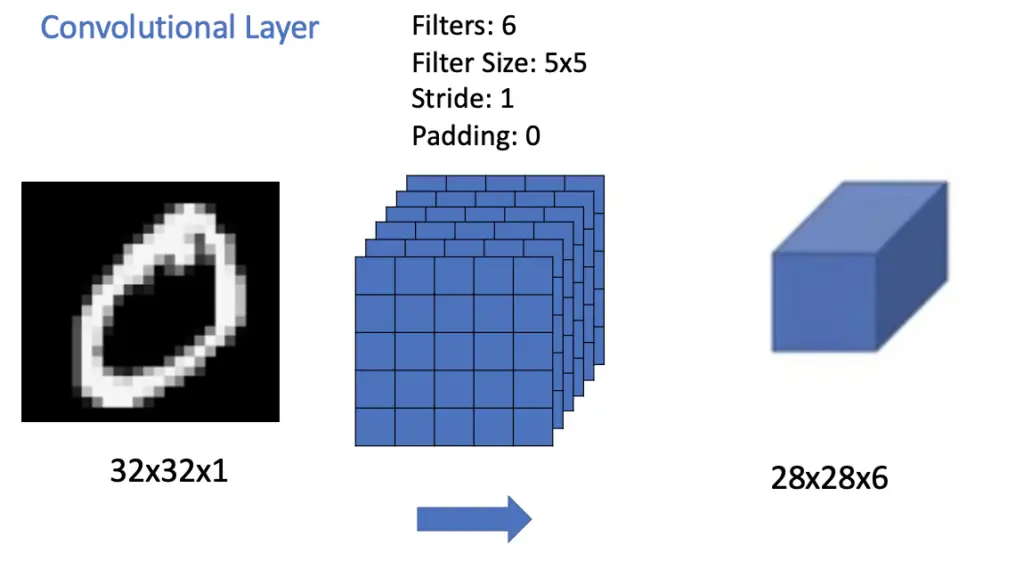
LeNet takes a 32×32 grayscale image as an input which means it does not have multiple color channels. The network was trained to recognize handwritten digits on the MNIST dataset. The image is passed to a convolutional layer with 6 filters, a filter size of 5×5, and a stride of 1, and no padding. Due to the six 5×5 filters, the result is a feature map with dimensions equal to 28x28x6. We also call these multidimensional data objects that are passed between layers tensors.

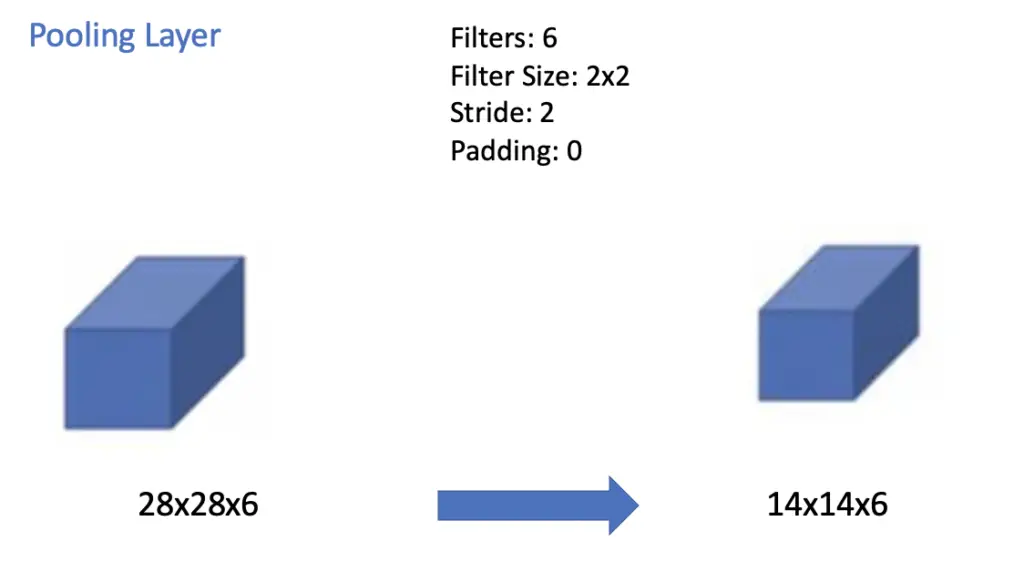
The feature map is passed to a pooling layer. The pooling filter has a dimension of 2×2 and is slid across the 6 channels produced by the convolutional layer using a stride of 2. Accordingly, the feature map shrinks by half along the vertical and horizontal dimensions to 14x14x6. LeNet applied average pooling, while most modern implementations mainly rely on max pooling.

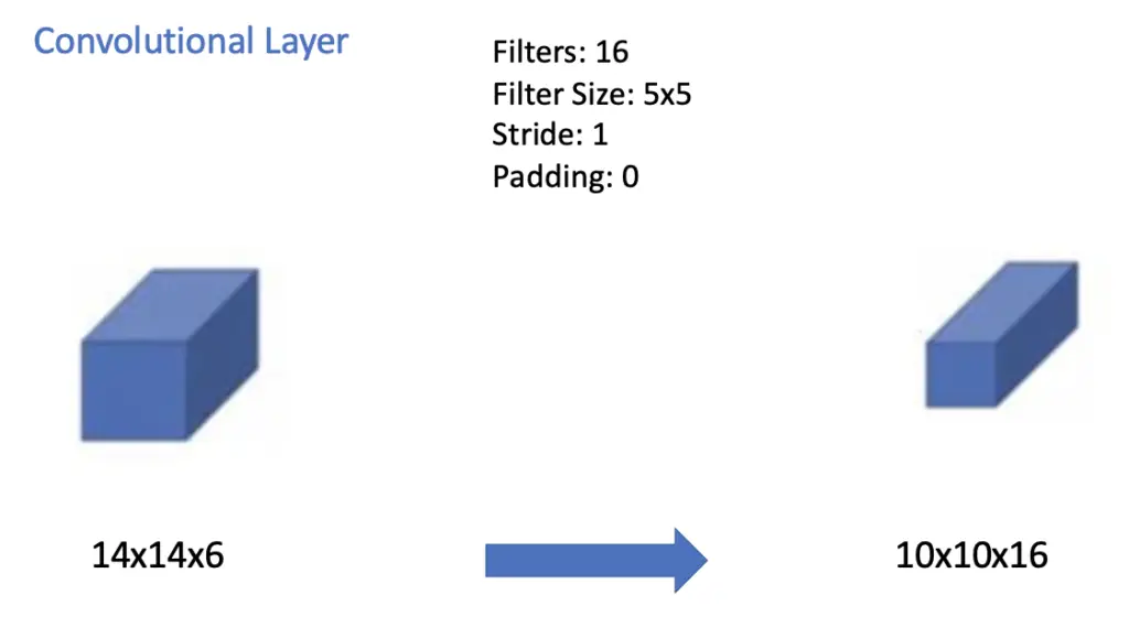
The next convolutional layer applies 16 filters with a size of 5×5, a stride of 1, and no padding. The output along the horizontal and vertical dimensions shrinks by 5-1 to 10×10 while the number of channels of the output map goes up to 16.

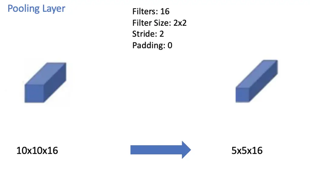
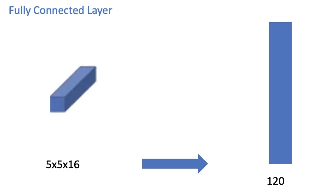
The convolutional layer is immediately followed by another average pooling layer using a filter size of 2×2 and a stride of 2. The result is a feature map with a dimensionality of 5x5x16.

The pooling layer is followed by a fully connected layer of 120 neurons. Each of these neurons connects to each of the 5x5x16 = 400 nodes in the previous layer.

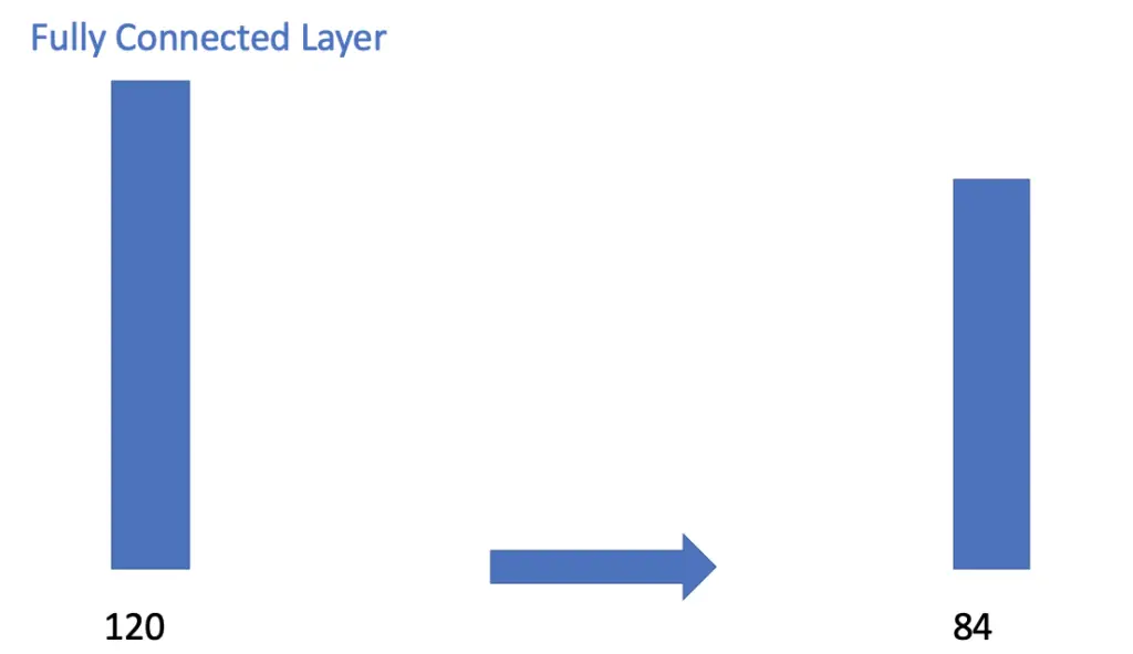
Next, we have another traditional fully connected layer that reduces down to 84 nodes.

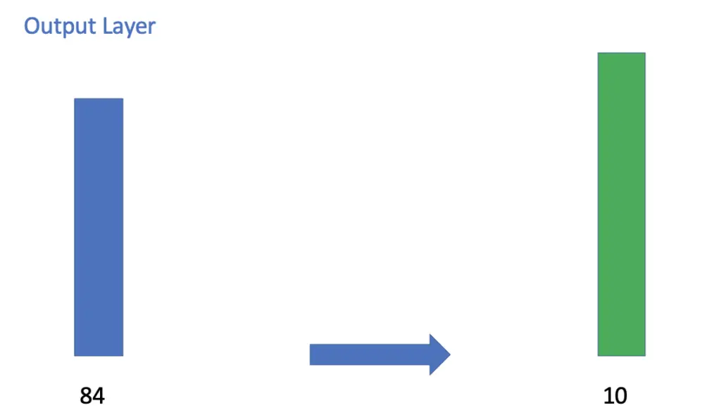
The fully connected layer finally connects to the output layer containing 10 nodes. Remember that LeNet was trained to distinguish between 10 different digits, which is why we have 10 output nodes.

This article is part of a blog post series on deep learning for computer vision. For the full series, go to the index.