Linear Regression in Python

This post is about doing simple linear regression and multiple linear regression in Python. If you want to understand how linear regression works, check out this post.

To perform linear regression, we need Python’s package numpy as well as the package sklearn for scientific computing. Furthermore, we import matplotlib for plotting.

import numpy as np
import matplotlib.pyplot as plt
from sklearn.linear_model import LinearRegression

Simple Linear Regression In Python

First, we generate tome dummy data to fit our linear regression model. We use the same data that we used to calculate linear regression by hand. Note that the data needs to be a NumPy array, rather than a Python list.

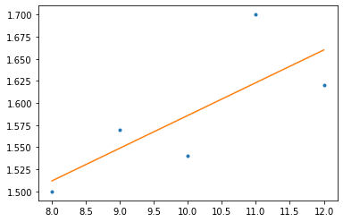
x = np.array([8,9,10,11,12])
y = np.array([1.5,1.57,1.54,1.7,1.62])

Simple Linear Regression in NumPy

If we want to do linear regression in NumPy without sklearn, we can use the np.polyfit function to obtain the slope and the intercept of our regression line. Then we can construct the line using the characteristic equation where y hat is the predicted y.

\hat y = kx + d

k, d = np.polyfit(x, y, 1)
y_pred = k*x + d

plt.plot(x, y, '.')
plt.plot(x, y_pred)

Simple Linear Regression in SKLearn

Python’s goto package for scientific computing, SciKit Learn, makes it even easier to fit a regression model.

First, we need to create an instance of the linear regression class that we imported in the beginning and then we simply call fit(x,y) on the created instance to calculate our regression line.

reg = LinearRegression()
reg.fit(x, y)

If we run the code like this, it will return a value error “Expected 2D array, got 1D array instead:”. Luckily Python gives us a very useful hint of what has gone wrong. The reason for this error is that the LinearRegression class expects the independent variables to be presented as a matrix with 2 dimensions with columns representing independent variables and rows containing observations. Here we only have one independent variable, and thus our vector only has one dimension. We can fix this error by reshaping x. If we print the shape of x we get a (5, 1) 2D array, which is Python-speak for a matrix, rather than a (5,) 1D array, a vector.

x = np.array([8,9,10,11,12]).reshape((-1, 1))
print(x.shape)

#fit the model to the data
reg.fit(x, y)

Now that we’ve successfully constructed our regression model, we can obtain several parameters such as the coefficient of determination, the slope, and the intercept.

#Coefficient of determination
r_squared = reg.score(x,y)
print(r_squared)

#slope
slope = reg.coef_
print(slope)

#intercept
intercept = reg.intercept_
print(intercept)

Finally, we can use the fitted model to predict y for any value of x.

y_pred = reg.predict(x)
print(y_pred)

We can further calculate the residuals, the difference between the actual values of y and the values predicted by our regression model. If we square the differences and sum them up, it gives us the sum of squared residuals

#SSR
residuals = y - y_pred

SSR = np.sum(residuals**2)
print(SSR)       

Note that Python vectorizes operations performed on vectors. All we have to do is write y – y_pred and Python calculates the difference between the first entry of y and the first entry of y_pred, the second entry of y, and the second entry of y_pred, etc.

That’s it for simple linear regression. For a complete overview over SciKit’s linear regression class, check out the documentation.

Multiple Linear Regression in Python

Until now we’ve played with dummy data. For this example, we are finally going to use a real dataset. We will use the diabetes dataset which has 10 independent numerical variables also called features that are used to predict the progression of diabetes on a scale from 25 to 346. The data is included in SciKitLearn’s datasets.

First, we need two additional imports:

from sklearn import datasets
import pandas as pd

Next, we import the diabetes dataset and assign the independent data variables to X, and the dependent target variable to y.

dataset = datasets.load_diabetes(as_frame=True)
x = dataset.data
y = dataset.target

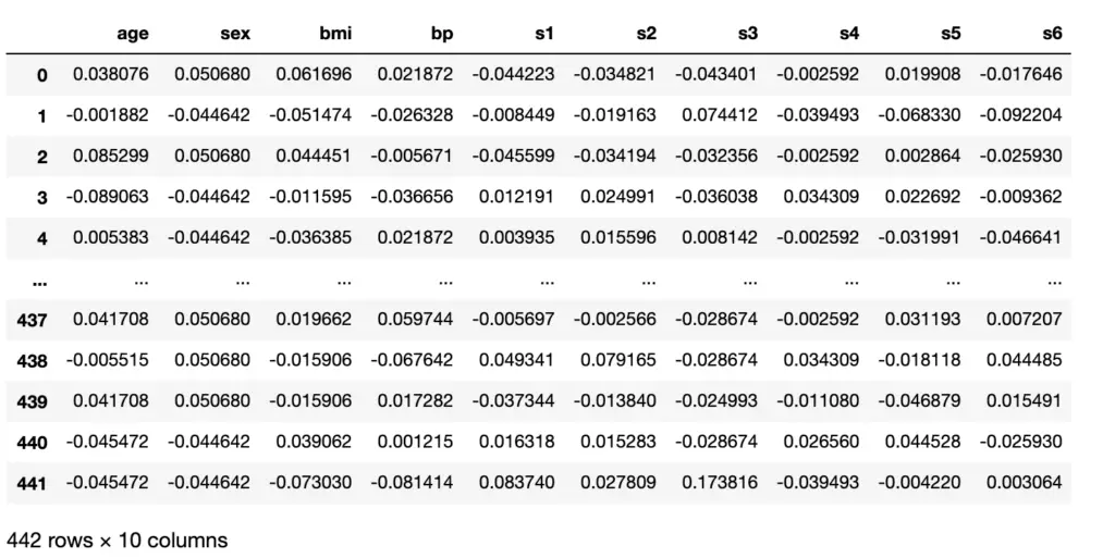
If you print the shape, you’ll see that X is a matrix with 442 rows and 10 columns, while y is a vector with 442 rows. The parameter “as_frame=True” imports the dataset as a data frame using the Pandas library instead of a NumPy array. Pandas makes visualizations easier and automatically imports the column headers. Let’s print X to see what I mean.

X

Next, we should check whether there are any missing values in the data. Null values can lead to nifty bugs that are sometimes hard to track down. So better be safe than sorry. The following code snippet checks for NA values, which is Python syntax for null values.

X.isna().sum()

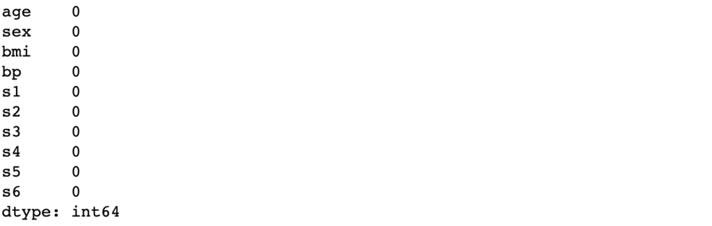
Things look good. Note, that when dealing with a real dataset I highly encourage you to do some further preliminary data analysis before fitting a model. At a minimum, you should check some elementary statistics such as the mean, minimum and maximum values and how strongly your independent features are correlated. In most cases, it is advisable to identify and possibly remove outliers, impute missing values, and normalize your data. But these operations are beyond the scope of this post, so we’ll build our regression model next.

First, we split our dataset into a large training and a smaller test set. Scikit Learn has its own function for randomly splitting a dataset, but we are going to just chop off the last 42 entries.

X_train = X[:400]
y_train = y[:400]
X_test = X[400:]
y_test = y[400:]

We’ll adopt the convention that X (capitalized) denotes a set of several independent variables, while x is a single independent variable.

Now we can fit our model as before. Only this time we have a matrix of 10 independent variables so no reshaping is necessary.

reg = LinearRegression()
reg.fit(X_train, y_train)

If you print the slope and the intercept, you’ll realize that Scikit learn will give you an array of ten slopes. Since we have multiple independent variables, we are not dealing with a single line in 2 dimensions, but with a hyperplane in 11 dimensions. Every independent variable has a different slope with respect to y.

#slope
slope = reg.coef_
print(slope)

#[[   5.02597344 -238.41461528  521.63399624  299.94110951 -752.12376074
#   445.15341214   83.51201877  185.57718337  706.4729074    88.68448421]]
   

#intercept
intercept = reg.intercept_
print(intercept)

#[152.72942545]

Ultimately, we want the fitted model to make predictions on data it hasn’t seen before. For this purpose, we’ve split the data into a training and a test set.

y_pred = reg.predict(X_test)

The predictions themselves do not help us much further. To evaluate the model we calculate the coefficient of determination and the mean squared error (the sum of squared residuals divided by the number of observations).

#Coefficient of determination
r_squared = reg.score(X_test,y_test)
print(r_squared)

#0.6985749009402125

#MSE
residuals = y_test - y_pred
SSR = np.sum(residuals**2)

print(SSR / len(y_test))

#1668.7496675899772

Since the predict function has given us y_pred as a 2D array of shape = (42,1), we wrote y_pred[:, 0] in line 8 to select all rows and the first column explicitly to get a 1D array of shape (42, ). If you don’t do this, you won’t get an error but a crazy high value.

To make sure your model is solid, you also need to test the assumptions that linear regression analysis relies upon. In a simple regression model, just plotting the data often gives you an initial idea of whether linear regression is appropriate. Since we are in 11-dimensional space and humans can only see 3D, we can’t plot the model to evaluate it visually.
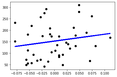
But you can plot each x value individually against the y-value.

Here is an example how to do this for the first independent variable.

x_train = X_train.values[:,0].reshape(-1, 1)
x_test = X_test.values[:,0].reshape(-1, 1)

simple_reg = LinearRegression()
simple_reg.fit(x_train, y_train)
y_pred = simple_reg.predict(x_test)

plt.scatter(x_test, y_test,  color='black')
plt.plot(x_test, y_pred, color='blue', linewidth=3)

If we extract a single column from X_train and X_test, pandas will give us a 1D array. Since the regression model expects a 2D array and we cannot reshape it directly in pandas, we extract the values as a NumPy array before we extract the column and reshape it into a 2D array.

Summary

We’ve learned to perform simple linear regression and multiple linear regression in Python using the packages NumPy and SKLearn. Regression analysis is a vast topic. There are several methods for selecting features, identifying redundant ones, or combining several features into a more powerful one. These methods are beyond the scope of this post, though, and need to wait until another time.