Regularization in Machine Learning

In this post, we introduce the concept of regularization in machine learning. We start with developing a basic understanding of regularization. Next, we look at specific techniques such as parameter norm penalties, including L1 regularization and L2 regularization, followed by a discussion of other approaches to regularization.

What is Regularization?

In machine learning, regularization describes a technique to prevent overfitting. Complex models are prone to picking up random noise from training data which might obscure the patterns found in the data. Regularization helps reduce the influence of noise on the model’s predictive performance.

Generally speaking, the goal of a machine learning model is to find patterns in data and apply the knowledge about these patterns to make predictions on different data from a similar problem domain.
In addition to noise, every dataset also contains random fluctuations with no explanatory value.

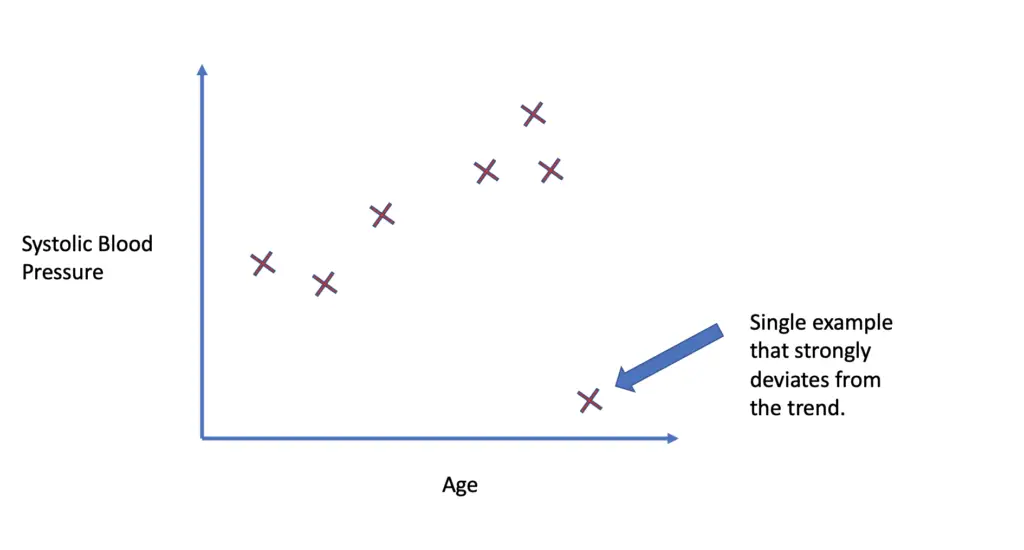
Assume you are trying to predict blood pressure using such factors as age, alcohol consumption, and history of smoking. Generally, higher age, drinking, and smoking are correlated with higher blood pressure. So there is a pattern that the model can pick up. Nevertheless, there may be some old individuals in your dataset who smoke and drink but have below-average blood pressure. This deviation from the pattern cannot be explained by our predictors. We treat it as noise.

Machine learning models might pick up some of that noise in a process known as overfitting. Even single examples that deviate significantly from the pattern known have the potential to change the model’s understanding of the pattern significantly. These examples are also known as outliers.

Imagine you have an outlier in your blood pressure training dataset (for example, an 80-year-old man who has been smoking and drinking his entire life but only has a blood pressure of 125/70).

If we fit a complex non-linear model without regularization, we might end up with a polynomial function that fits the training data perfectly well.

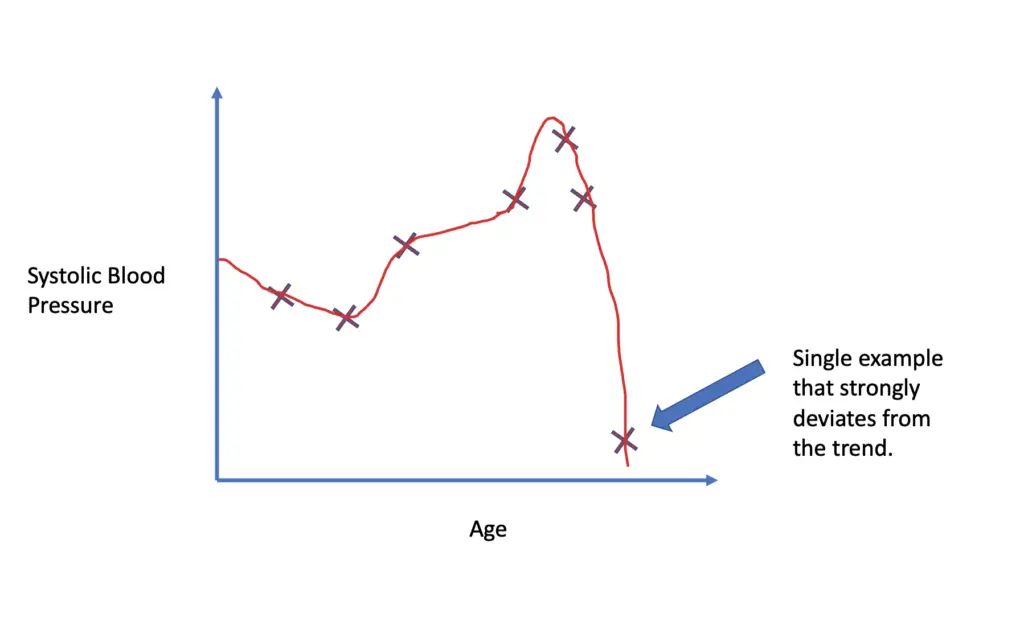
In other words, the model thinks that a blood pressure of 125/70 for an 80-year-old smoking alcoholic is part of the pattern. If it finds an individual with similar characteristics in the test set, it might predict unrealistically low blood pressure.

To prevent the model from picking up this kind of noise that obscures the underlying pattern, we can use regularization.
Note that before you apply regularization, you should try to denoise the data (for example, by removing outliers) and make sure you have picked an appropriate model.

Regularization Through the Cost Function

Learning complex patterns in datasets requires sophisticated models that are capable of representing higher-order mathematical functions. But the higher-order polynomials in those functions that enable models to learn complex patterns also lead to greater variance and therefore make the models more susceptible to overfitting.

The basic idea of regularization through the cost function is to penalize the higher-order polynomials to the extent that the model is still able to represent the patterns in the data but doesn’t get distracted by noisy deviations from the pattern. You essentially try to prevent the model from becoming overly complex.

How do we do this in practice?

At a large enough sample size, noise follows a Gaussian distribution. This means that large random deviations from the pattern are much more unlikely than smaller ones.
In a regression setting, we use this principle when calculating the loss of a machine learning model using the mean squared error. We add up the sums of the squared differences between the predictions produced by the model \hat f(x_i) and the actual values y_i observed to get to the cost J. The model \hat f(x_i) is parameterized by a set of model parameters θ. Those are the parameters we want the model to adjust in regularization. We can calculate the loss with respect to the parameters θ as follows.

J(\theta) = \sum_{i=1}^n (\hat f_{\theta}(x_i) - y_i)^2

Squaring the difference between the predicted value and the actual value disproportionately increases the error for large differences. The model should reduce the loss so it will be especially sensitive to large deviations.
With regularization, we can increase the impact of noisy deviations from the pattern even more by adding a term to the loss that is a function Ω of the parameters θ we want to regularize.

J(\theta) = \sum_{i=1}^n (\hat f_{\theta}(x_i) - y_i)^2 + \lambda\Omega(\theta)

The letter λ represents a hyperparameter which we can adjust to increase or decrease the impact of regularization. If we set it to 0, the model won’t be regularized at all.
In machine learning, two types of regularization are commonly used. L2 regularization adds a squared penalty term, while L1 regularization adds a penalty term based on an absolute value of the model parameters. In the next section, we look at how both methods work using linear regression as an example.

Regularization in Linear Regression

To illustrate how regularization works concretely, let’s look at regularized linear regression models. The principle is similar to the generic form shown above. Since we have multiple parameters θ, we need to sum not only over the n training examples but also over the number of parameters p. In a simple linear regression model, the first parameter is the intercept, while all other parameters in θ are multiplied by the predictors x.

J(\theta) = \sum_{i=1}^n ( y_i - \theta_0 - \sum_{k=1}^px_{ik} \theta_k)^2

Using this method, we can either apply L1 or L2 regularization

L2 Regularization (Ridge)

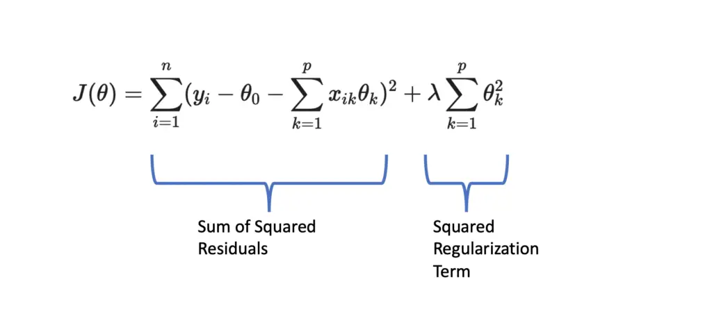
With L2 regularization, we add a regularization term that consists of the squared sum of all parameters θ multiplied by the hyperparameter λ.

J(\theta) = \sum_{i=1}^n ( y_i - \theta_0 - \sum_{k=1}^px_{ik} \theta_k)^2 + \lambda \sum_{k=1}^p \theta_k^2

This is also known as ridge regression.

L1 Regularization (Lasso)

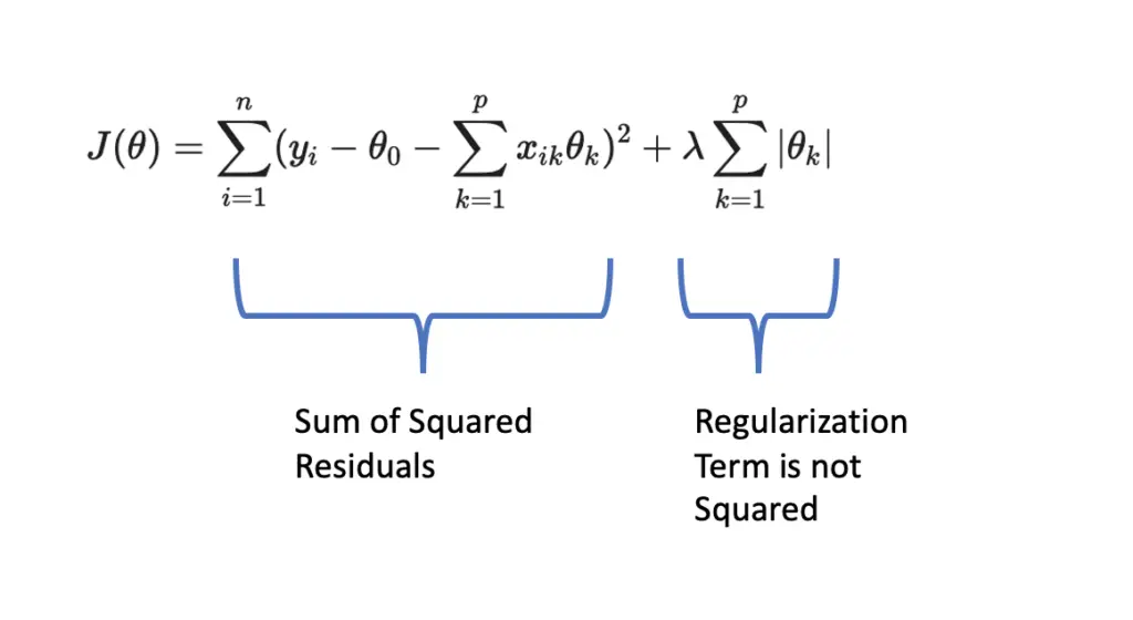
L1 regularization is very similar to L2 regularization, but there is one subtle difference. Rather than adding the squared sum of all parameters, we just add the sum of absolute values.

J(\theta) = \sum_{i=1}^n ( y_i - \theta_0 - \sum_{k=1}^px_{ik} \theta_k)^2 + \lambda \sum_{k=1}^p |\theta_k|

Ridge Regression vs Lasso

Even though the difference between ridge regression and the lasso (L2 regularization and L1 regularization) looks small, they produce very different effects.
Ridge regression regularizes by a factor that is proportional to the sum of squared residuals (the sum of the squared differences between predicted and actual values) because the regularization term is also squared.
In practice, this means that ridge regression can shrink the weight given to parameters, but it cannot altogether eliminate them (set them to zero).

When applying the L1 norm, the regularization term is not squared. Accordingly, it does not grow proportionally to the sum of squared residuals. In practice, this means if lambda is set sufficiently large, the regularization term and thus the cost can grow so large that the model sets parameter values to zero to get the cost under control (setting the parameters θ equal to zero eliminates the regularization term).

Thus, contrary to the L2 penalty in ridge regression, the L1 penalty in the lasso can be used to eliminate parameters.

For a more detailed explanation of how exactly this works, I recommend watching this video.

Further Regularization Methods

Besides the regularization techniques that build on the cost function, there are several other ways to reduce the variance that are often called regularization.

Ensemble Learning

Ensemble learning is about combining the outputs of several algorithms that have been trained individually. I won’t discuss more details here because ensemble learning is a vast subfield of machine learning that merits at least a separate article. Just note that ensemble learning itself does not necessarily reduce overfitting but can even increase it.

K-Fold Cross Validation

Another popular approach often used when little training data is available is cross-validation. You essentially split your dataset into k different non-overlapping subsets. Then you retain one of the subsets as a validation set and train your model on the remaining subsets. The process is repeated until each subset has served as the validation set. Ultimately, you’ll end up with k models that you can compare.
By comparing the models that have each been evaluated on a different subset of the training data, you get a more robust estimate of how well your model generalizes to new data.
Note that this method does not directly reduce overfitting. Rather, it can help you detect overfitting. If you only evaluate your model on one small subset of the data, great performance could be due to chance.

There are several more regularization methods that only apply to certain machine learning methods, such as dropout in neural networks or entropy regularization in reinforcement learning. I will discuss them in the context of these methods.

Summary

Regularization is a technique to reduce overfitting in machine learning.

We can regularize machine learning methods through the cost function using L1 regularization or L2 regularization. L1 regularization adds an absolute penalty term to the cost function, while L2 regularization adds a squared penalty term to the cost function.

Besides cost-function-based approaches, there are other model-specific approaches such as dropout in neural networks. Other approaches such as ensemble learning and cross-validation are also sometimes used to help reduce overfitting.