The Poisson Distribution

We introduce the Poisson distribution and develop an intuitive understanding of its uses by discussing examples and comparing the Poisson distribution to the binomial distribution.

With the Poisson distribution, we can express the probability that a certain number of events happen in a fixed interval.

Poisson Distribution Examples

The Poisson distribution is useful in any scenario where you want to model the occurrence of independent events happening at a certain rate.

For example, suppose you want to optimize traffic flows in your city. There is a critical intersection, which cannot handle more than 100 cars in a 10-minute window. You can use the Poisson distribution to calculate the probability that 100 cars pass by a certain point in a 10-minute window.

The Poisson distribution is also used to model the decay of radioactive compounds or the rate of significant events such as market crashes in finance.

Poisson Distribution Formula

Central to the Poisson distribution is the parameter lambda, which describes the rate at which events are happening. For a Poisson random variable X, lambda is simply the mean number of events x happening per interval. The probability mass function is

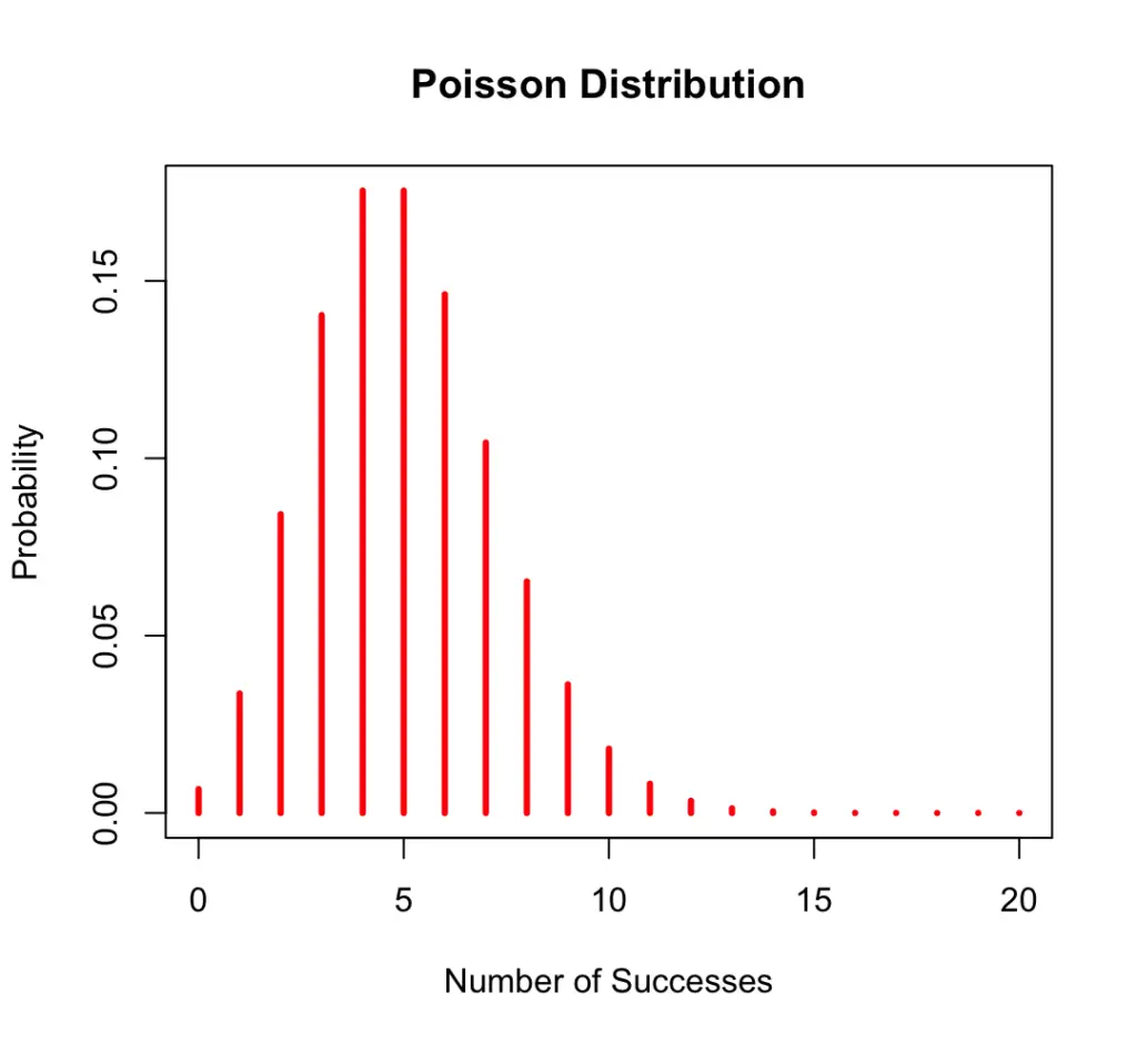
f(x, \lambda) = P(X=x) = \frac{\lambda^x e^{-\lambda}}{x !}

Let’s say you are looking at an intersection and expect cars to take a left turn at a rate of 5 per minute. You could calculate the probability of observing 3 cars turning left by using the Poisson distribution.

P(X=x) = \frac{5^3 e^{-5}}{3 !} = 0.14

We can plot the probability mass function. Naturally, the probability that x equals 5 is the highest.

The expected value and variance of a poisson random variable are both equal to lambda.

Poisson vs Binomial

The Poisson distribution may be a better fit for certain problems that could also be modeled using a binomial distribution.

Recall that the binomial distribution models the probability of observing x events out of n trials.

P(X=x) = {n \choose x}p^x(1-p)^{n-x} 

In the Poisson distribution, we can think of the parameter lambda as the product of the probability and the number of trials.

\lambda = n \times p

Let’s try to model the previous situation with cars taking a left turn with a binomial distribution to understand why the Poisson distribution is a better fit in this case.

Applying the binomial probability mass function to the intersection problem, we could say n is the total number of cars passing through the intersection within an hour while x is the number of cars taking a left turn.

But wait, the previous example only gave us the rate at which cars turn left. It did not give us the exact number of cars passing through the intersection. There is our first reason why the Poisson distribution is a better fit. It requires less information.

Let’s say for the sake of example, that there are 50 cars in one hour.

P(X=5) = {50 \choose 5}0.1^5(1-0.1)^{50-5} 

The next problem with the binomial distribution is that it only counts one event as a success. In this case, we count 5 cars turning left as a success. But we might as well have 4 or 6 cars turning left within that timeframe.

To account for all events, we could reduce the timeframe to an amount within which we can expect to only observe one car and then observe these timeframes sequentially. But that doesn’t solve our problem either. There could still be intervals of our new timeframe within which 0, 2,3, or more cars turn left.

If we really wanted to catch all the events, we would have to reduce the timeframe so much that the probability of observing even one event becomes infinitesimally small, essentially limiting towards zero. If we plug this into our formula for lambda, lambda will be zero.

\lambda = n \times 0

To prevent this from happening, we make n so large that it tends towards infinity.

This is the basic logic of the Poisson distribution. We make p so small and n so large that we don’t really have to care about them anymore.

With this knowledge in place, we can derive the Poisson distribution from the binomial distribution. First, we replace p with lambda over n.

p = \frac{\lambda}{n}

Then we perform some arithmetic.

P(X=x) = {n \choose x}p^x(1-p)^{n-x} 

\lim_{n \to \infty} \frac{n!}{x!(n-x)!}  (\frac{\lambda}{n}) ^x(1-\frac{\lambda}{n})^{n-x} 

\lim_{n \to \infty}\frac{n!}{(n-x)!} 
   \frac{1}{n^x}
\frac{\lambda^x}{x!} 
(1-\frac{\lambda}{n})^{n} 
(1-\frac{\lambda}{n})^{-x} 

Now, we are in a position to simplify terms:

\lim_{n \to \infty}(1-\frac{\lambda}{n})^{n} = e^{-\lambda}

\lim_{n \to \infty}(1-\frac{\lambda}{n})^{-x}  = 1

\lim_{n \to \infty}\frac{n!}{(n-x)!} 
   \frac{1}{n^x} = 1

Putting it all together:

\frac{\lambda^x e^{-\lambda}}{x!} 

If you compare it to the result from above, you’ll see that this is, in fact, the Poisson distribution.

Compared to the binomial, the Poisson distribution is more appropriate if we can observe events happening at a certain rate but without knowledge of the number of trials.

This post is part of a series on statistics for machine learning and data science. To read other posts in this series, go to the index.