Understanding Convolutional Filters and Convolutional Kernels

This post will introduce convolutional kernels and discuss how they are used to perform 2D and 3D convolution operations. We also look at the most common kernel operations, including edge detection, blurring, and sharpening.
A convolutional filter is a filter that is applied to manipulate images or extract structures and features from an image. Convolutional filters are typically used to blur or sharpen sections of an image or to detect edges in them.
Convolutional Filters
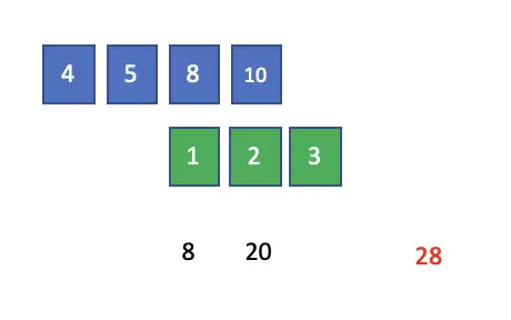
In the post on the convolution operation, I introduced the convolutional kernel as a grid containing numbers that we slide over another number grid to generate an output.
The convolutional filter is a multidimensional version of the convolutional kernel, although the two terms are often used interchangeably in the computer vision community.
2D Convolution
2D convolutions are essential for the processing of 2D data such as images. An image is basically a 2-dimensional grid of pixel values. Standard RGB images have pixel values ranging from 0 to 255 and three channels (red, green, and blue) which adds a third dimension. But to simplify things a bit, we only look at one channel, which leaves us with a 2D grid of pixels which is enough to represent grayscale images.

To manipulate images, we can convolve the image with a 2-dimensional kernel.
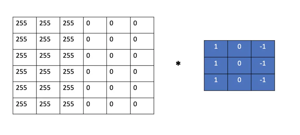
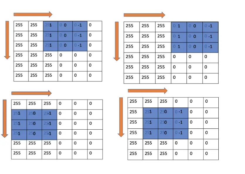
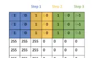
As you see in the image, the kernel, in this case, is a smaller 2D grid. To compute the convolution, we slide the kernel over the image and calculate the convolution across two dimensions.
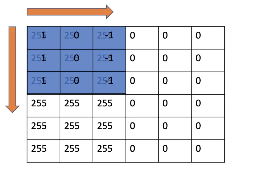
Starting in the upper-left corner, we slide the kernel over the image and perform an element-wise multiplication with the image followed by a summation.
1\times255 + 0\times255 +(-1)\times255 \\ + 1\times255 + 0\times255 +(-1)\times255 \\ +1\times255 + 0\times255 +(-1)\times255 \\ = 0
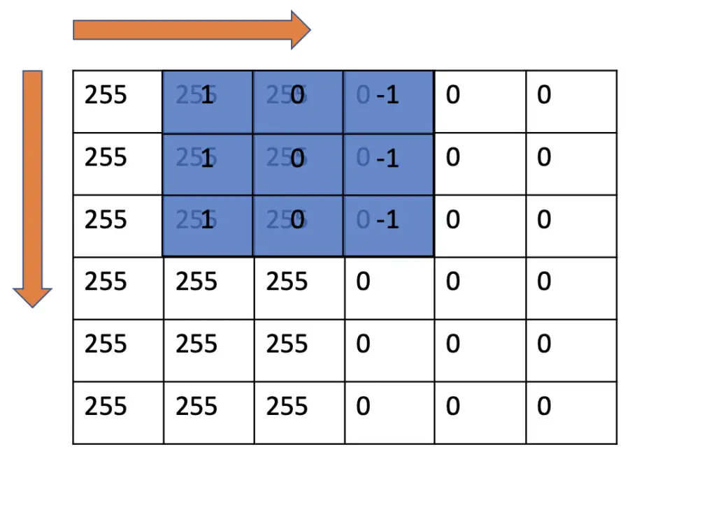
Next, we slide the kernel to the right and repeat the convolution operation.
1\times255 + 0\times255 +(-1)\times0 \\ + 1\times255 + 0\times255 +(-1)\times0 \\ +1\times255 + 0\times255 +(-1)\times0 \\ = 765
You continue this process, sliding the kernel to the right and downwards until you reach the lower-right corner. In each step, you convolve the kernel with the part of the image.
The results of the convolution operations can be neatly represented in a 4×4 matrix.
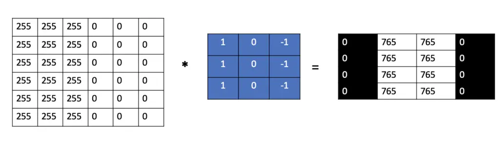
As you can see, the two columns in the center contain very high numbers, whereas the pixel values on the margins contain zeros. This indicates that there is a bright vertical edge running through the center. This particular kernel that we have used performs vertical edge detection. What type of operation the kernel performs depends on the numbers used in the kernel and their ordering. We will discuss different types of convolutional kernels later in this article.
Mathematical Representation of the 2D Convolution
Mathematically, we can represent the 2D convolution as follows:
(I * K) (i, j)= \sum_m \sum_n I(m,n)K(i-m,j-n)
This operation is commutative. As a consequence, we can flip the kernel and write it like this.
(K * I) (i, j)= \sum_m \sum_n I(i-m,j-n)K(m,n)
In many practical applications, cross-correlation is used instead of the convolution operation.
(K * I) (i, j)= \sum_m \sum_n I(i-m,j-n)K(m,n)
The cross-correlation is not commutative. In purely mathematical terms, this is an important distinction. But in practice, the distinction doesn’t really matter, which is why the term convolution is often used when referring to cross-correlation.
3D Convolution
When performing 3D convolution, you are sliding a 3-dimensional kernel over a 3-dimensional input. The kernel needs to have the same depth as the input. You calculate the convolution of each channel in the kernel with each corresponding channel in the image.
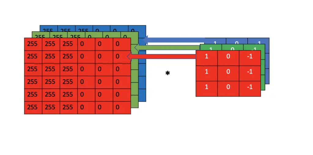
Essentially, you need to perform the 2D convolution operation three times over, and then you sum up the results to get the final kernel output.
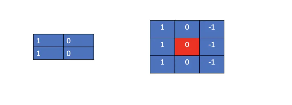
Why Do We Use Odd Kernels?
In the previous examples, we’ve used 3×3 kernels. While differently sized kernels are used, the size is almost always odd. The reason for using odd kernels is symmetry around the origin. If you are using an evenly sized kernel, there is no clear center point.
Sliding convolutional filters over an image allows you to manipulate an image in various ways. In the remainder of this post, we will go through some of the more commonly used convolutional filters and their effects.
Edge Detection Kernels
The kernel we’ve used above is a simple vertical edge detector known as the Prewitt Operator.
The Prewitt Operator
The Prewitt operator for vertical edge detection appears in the form of the following matrix.
\begin{bmatrix}
1 & 0 & -1 \\
1 & 0 & -1 \\
1 & 0 & -1 \\
\end{bmatrix}
If we apply the vertical Prewitt operator to a real image, the result looks like this.
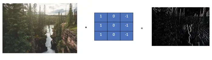
There is a strong vertical color contrast between the river and the cliffs, which is prominently visible.
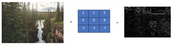
To apply horizontal edge detection, we can rotate the kernel by 90 degrees.
\begin{bmatrix}
1 & 1 & 1 \\
0 & 0 & 0 \\
-1 & -1 & -1 \\
\end{bmatrix}
Now, the horizontal edges are more visible.
The Sobel Operator
The Sobel operator emphasizes the edges more than the Hewitt operator by replacing 1’s in the central column with 2’s.
Here is the Sobel operator for vertical edge detection.
\begin{bmatrix}
1 & 0 & -1 \\
2 & 0 & -2 \\
1 & 0 & -1 \\
\end{bmatrix}
For horizontal edge detection, you can use the following kernel.
\begin{bmatrix}
1 & 2 & 1 \\
0 & 0 & 0 \\
-1 & -2 & -1 \\
\end{bmatrix}
The Laplacian Operator
The Laplacian filter is an approximation to the 2nd spatial derivative of the image. If that sounds confusing, don’t worry. In practice, it basically means that the Laplacian filter highlights areas where the intensity of the pixel values is changing drastically. Consequently, it is a very popular filter for detecting both horizontal and vertical edges at once.
The LaPlacian is most commonly approximated with the following filter.
\begin{bmatrix}
0 & 1 & 0 \\
1 & -4 & 1 \\
0 & 1 & 0\\
\end{bmatrix}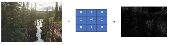
The filter is frequently combined with Gaussian blurring or smoothing as it amplifies the edges even more.
Smoothing and Blurring Kernels
Blurring is an important technique in image processing that makes the transition between different pixel values smooth rather than sharp. Therefore, the technique is also called smoothing. It is especially useful when you want to shrink the size of an image. Some sharp details will inevitably be lost. With smoothing, you can distribute the color transition over more pixels which preserves the edges even if the image is smaller overall.
Gaussian Filter
The Gaussian filter weighs intensities according to a normal or Gaussian distribution. A Gaussian distribution has the characteristic form of a bell curve. The curve peaks at the center and flattens out the further you get away from the center. Thus, the center of the filter contains the highest value while the values further away are smaller.
The following kernel is a discrete approximation to the Gaussian distribution.
\frac{1}{16}
\begin{bmatrix}
1 & 2 & 1 \\
2 & 4 & 2 \\
1 & 2 & 1\\
\end{bmatrix}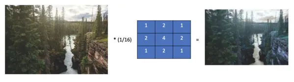
Box Filter
The box kernel is a simple filter that calculates the mean of the pixels in the area covered by the filter. This also has a smoothing effect.
Contrary to the Gaussian filter, which weighs pixels according to a normal distribution, the box filter weighs all pixels equally. The box filter is faster and easier to calculate than the Gaussian filter.
\frac{1}{9}
\begin{bmatrix}
1 & 1 & 1 \\
1 & 1 & 1 \\
1 & 1 & 1\\
\end{bmatrix}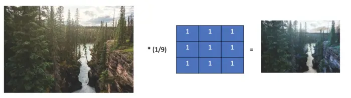
Sharpen Filter
Filters to sharpen images accentuate edges. They essentially do the opposite of blurring. A common kernel for sharpening images is the following one.
\begin{bmatrix}
0 & -1 & 0 \\
-1 & 5 & -1 \\
0 & -1 & 0\\
\end{bmatrix}
Conclusion
Convolutional Kernels and Filters are the building blocks of many computer vision applications. More advanced algorithms such as Canny edge detection build on combining several convolutional kernel types such as those used for smoothing and edge detection. Kernels are also at the heart of the most advanced computer vision technologies, such as convolutional neural networks used in deep learning.
This article is part of a blog post series on deep learning for computer vision. For the full series, go to the index.
