Weight Decay in Neural Networks

What is Weight Decay

Weight decay is a regularization technique in deep learning. Weight decay works by adding a penalty term to the cost function of a neural network which has the effect of shrinking the weights during backpropagation. This helps prevent the network from overfitting the training data as well as the exploding gradient problem.

In neural networks, there are two parameters that can be regularized. Those are the weights and the biases. The weights directly influence the relationship between the inputs and the outputs learned by the neural network because they are multiplied by the inputs. Mathematically, the biases only offset the relationship from the intercept. Therefore we usually only regularize the weights.

Weight Decay with the L2 Norm

The L2 penalty is the most commonly used regularization term for neural networks. You apply L2 regularization by adding the squared sum of the weights to the error term E multiplied by a hyperparameter lambda that you pick manually.

C = E + \frac{\lambda}{2n}  \sum_{i=1}^{n}w_i^2

The full equation for a cost function would look like this, where the function L represents a loss function such as cross-entropy or mean squared error.

C(w, b) = \frac{1}{n} \sum_{i=1}^{n} L(\hat y_i, y_i) + \frac{\lambda}{2n}  \sum_{i=1}^{n}w_i^2

But how does this term shrink the weights during backpropagation? To understand this, let’s have a look at the cost function for a single training example. This allows us to remove the summation and to average over n examples. For the sake of the demonstration, we also ignore b since it is not regularized.

During backpropagation, we calculate the gradient of the cost function with respect to w.

\frac{\partial C}{\partial w_i} =  \frac{\partial E}{\partial w_i} + \frac{\partial}{\partial w_i} (\frac{\lambda}{2}  w_i^2)

Differentiating the penalty term with respect to the weight gives us the following outcome (we originally divided λ by 2 so it would cancel out the 2 from the differentiation)

\frac{\partial C}{\partial w_i} =  \frac{\partial E}{\partial w_i} +  \lambda  w_i

When performing updates to the weight during gradient descent, we subtract the gradient multiplied by the learning rate α from the weight.

w_{i_{updated}} = w_i - \alpha \frac{\partial C}{\partial w_i}

w_{i_{updated}} = w_i - \alpha (\frac{\partial E}{\partial w_i} +  \lambda  w_i)

So the regularized weight update shrinks the weights by the gradient plus a penalty term rather than by the gradient alone (in practice, you scale both by a learning rate α to get gradient descent to converge).

Weight Decay with the L1 Norm

When applying weight decay with the L1 norm, you use the absolute value of the sum of the weights rather than their squared value.

C = E + \frac{\lambda}{2n}  \sum_{i=1}^{n} ||w_i|]

The crucial difference between L1 and L2 regularization is that the L1 norm can completely eliminate parameters by setting the weights equal to zero.

For an intuitive understanding of why this is the case, consider that squaring terms that are smaller than zero, such as the weights, will lead to a faster shrinkage of the penalty term. The closer the weight gets to zero, the more the penalty term will shrink relative to the weight. The L1 penalty is not squared. Instead, it subtracts a bigger constant value from the weight in every iteration that can reach 0.

As a consequence, L1 regularized weight matrices end up becoming sparse, which means many of its entries equal zero.

Why Does Shrinking the Weights Help Prevent Overfitting?

In practice, the dataset you use to train a neural network will usually contain patterns that are reflective of the problem for which the network is being trained as well as random fluctuations that have no explanatory value.
Our goal is to learn as much about the patterns while getting the network to ignore the random fluctuations.

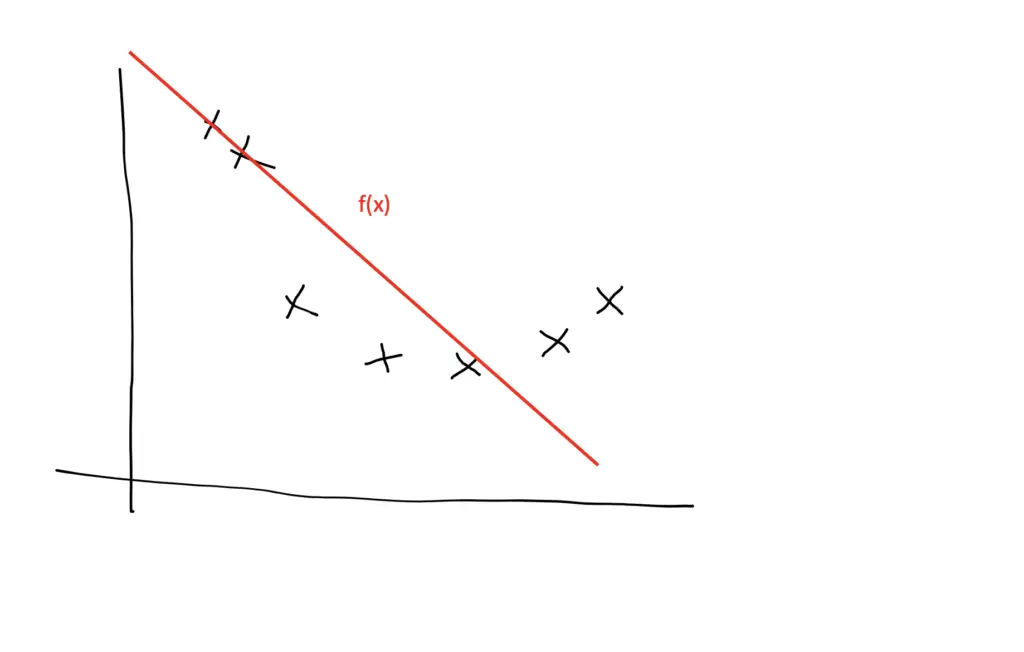
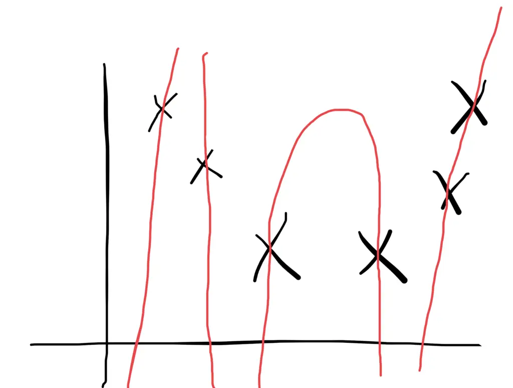
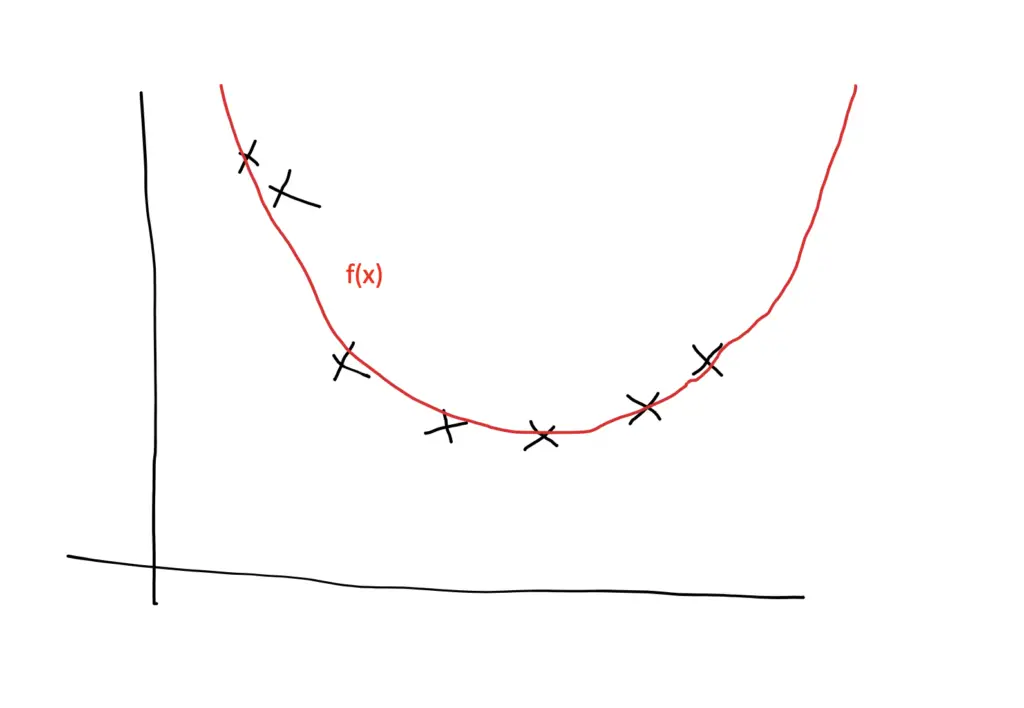
The more big weights we have, the more active our neurons will be. They will use that additional power to fit the training data as closely as possible. As a consequence, they are more likely to pick up more of the random noise.

Shrinking the weights has the practical effect of effectively deactivating some of the neurons by shrinking their weights close to zero. The larger you set the regularization parameter lambda, the smaller the weights will become. But note that contrary to L1 regularization, L2 regularization doesn’t completely set the weights equal to zero. So when using L2 regularization, the neurons technically are still active, but their impact on the overall learning process will be very small.

With its reduced power, the network needs to focus more on patterns that frequently occur throughout the dataset and are thus more likely to be a manifestation of the actual problem the network is trying to model. As a result, the model will also become smoother, meaning that the outputs change more slowly in response to changing inputs.

Weight Decay in TensorFlow

First, we have to import the layers and regularizers from TensorFlow.

import tensorflow as tf
from tensorflow.keras.layers import Dense
from tensorflow.keras.regularizers import l2

Regularization in Tensorflow is fairly straightforward. You only need to set the parameter “kernel_regularizer” on the layer that you want to regularize. to the selected loss along with the regularization parameter.

Here, we are creating a Dense layer with L2 regularization and a regularization parameter of 0.1:

Dense(128, kernel_regularizer=l2(0.1), activation="relu")

Similaryl, we can apply L1 regularization:

Dense(128, kernel_regularizer=l1(0.1), activation="relu")

We can string several regularized regularized layers together into a simple neural network using the sequential API. Here our input data has 3 dimensions, which is why we set the input_shape to 3 in the first dense layer. We call the regularization parameter “lambd” since lambda is a reserved keyword in Python.

lambd = 0.1
model = Sequential([
        Dense(64, kernel_regularizer=l2(lambd), activation="relu", input_shape=(4,)),
        Dense(128, kernel_regularizer=l2(lambd), activation="relu"),
        Dense(128, kernel_regularizer=l2(lambd), activation="relu"),
        Dense(128, kernel_regularizer=l2(lambd), activation="relu"),
        Dense(64, kernel_regularizer=l2(lambd), activation="relu"),
        Dense(64, kernel_regularizer=l2(lambd), activation="relu"),
        Dense(64, kernel_regularizer=l2(lambd), activation="relu"),
        Dense(3, activation='softmax')
    ])

This article is part of a blog post series on the foundations of deep learning. For the full series, go to the index.