Bernoulli Random Variables and the Binomial Distribution in Probability

In this post, we develop an understanding of Bernoulli random variables and the binomial distribution. We introduce scenarios that follow the binomial distribution and learn how it relates to the normal distribution.

The Bernoulli Distribution

A Bernoulli random variable can be used to model the probability of a system whose outcome can only result in a success or failure. Accordingly, a Bernoulli random variable can only take two values: 0 and 1 or failure and success. For example, the outcome of a coin flip can be modeled using a Bernoulli random variable.

The two values a Bernoulli random variable X can assume are usually denoted using x, and 1-x. The probabilities of these two outcomes need to sum to 1. Accordingly, the probabilities are denoted as p and 1-p.

The probability mass function that describes a Bernoulli trial, known as the Bernoulli distribution, can be described mathematically in the following formula.

P(X = x) = p^x(1-p)^{1-x}

If we plug our fair coin toss scenario into the formula, we would have a probability of 0.5 for each outcome of X.

Let’s say the probability of obtaining a head is 1 and obtaining a tail is 0.

x \in \{0,1 \}\\
p_{Head} = p = 0.5 \\
p_{Tail} = 1-p = 0.5

P(X = x) = 0.5^1 0.5^0 = 0.5

Unsurprisingly, the probability of getting a head is 0.5

The Binomial Distribution

The outcome of repeated Bernoulli trials (like flipping a coin multiple times in a row) follows a binomial distribution. The binomial distribution is thus a generalized form of the Bernoulli distribution.

It describes the probability of observing a certain number x occurrences out of a total of n trials.

P(X=x) = {n \choose x}p^x(1-p)^{n-x} = \frac{n!}{x!(n-x)!} p^x(1-p)^{n-x} 

For example, if I throw a coin 2 times, what is the probability of getting one head?

We can describe this scenario using a binomial distribution using the following parameters.

n = 3\\
x = 2\;where \; x \in \{0,1,2,3\}\\
p_{Head} = p = 0.5 \\
p_{Tail} = 1-p = 0.5

P(X=2) = \frac{3!}{2! \times 1!} 0.5^2 \times 0.5^1 = 0.375

Properties of the Binomial Distribution

The mean and variance of the binomial distribution are

E(x) = n \times p

V(x) = n\times p (1-p)

In other words, if you were to throw coin three times, the expected value or mean of all coin throws would simply be the number of throws times the probability of getting a successful outcome (which we defined as head = 1).

E(x) = 3 \times 0.5 = 1.5

For the standard deviation we need to multiply again by the probability of the non-successful outcome (tails = 0)

V(x) = 3 \times 0.5 \times 0.5 = 0.75

So far we have assumed fair outcomes where the probability is evenly split. But there are scenarios, where the probability distribution is skewed towards one outcome. For example, if the coin wasn’t fair and had a 0.6 probability of success, variance, and expected value would change accordingly.

E(x) = 3 \times 0.6 = 1.8

V(x) = 3 \times 0.6 \times 0.6 = 1.8

The probability mass function of the binomial distribution looks like a bell curve with the location of its peak as well as its width being determined by the probability of the single outcome and the number of trials.

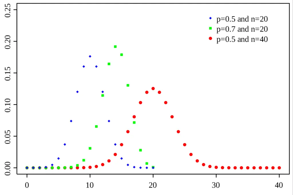
In other words, the mean and variance of the binomial distribution form a normal distribution.

Summary

We introduced the Bernoulli distribution and the binomial distribution. We’ve developed an understanding of scenarios that follow the binomial distribution and learned how it relates to the normal distribution.

This post is part of a series on statistics for machine learning and data science. To read other posts in this series, go to the index.