The Fundamental Theorem of Calculus and Integration

In this post, we introduce and develop an intuitive understanding of integral calculus. We learn how the fundamental theorem of calculus relates integral calculus to differential calculus.

Integration is the reverse operation of differentiation. Together they form a powerful toolset to describe non-linear functions. While differentiation enables us to describe the gradient or rate of change of a function, integration allows us to calculate the area under a non-linear function. The fundamental theorem of calculus neatly ties the two operations together.

I’ve discussed differential calculus and its applications at length in previous posts. Integral calculus is important in areas like statistics and machine learning if you are dealing with continuous rather than discrete functions. However, very few practical applications require you to solve integrals analytically by hand. Rather than teaching arcane rules, I will try to provide a brief intuitive understanding of integration before discussing the fundamental theorem of calculus.

What is Integral Calculus

Assume you gain an approximate estimation of the area under a curve f(x) for a certain interval using nothing but simple algebra. You can split the area into n areas of equal width. At each point i, you evaluate the function f(x). This gives you the length of the rectangle at that point. You also choose an arbitrary width Δx (equal for each rectangle).

length_i = f(x_i)\\
width_i = Δx_i\\

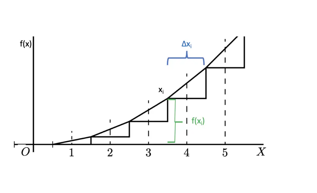
Now you can calculate the area of each rectangle by simply multiplying the width with the height. You obtain the estimated area of f(x) by summing all rectangle areas.

S = \sum_{i=1}^{n}f(x_i)Δx_i

We can get a closer estimate of the real area under the curve by reducing the width Δx and creating more rectangles.

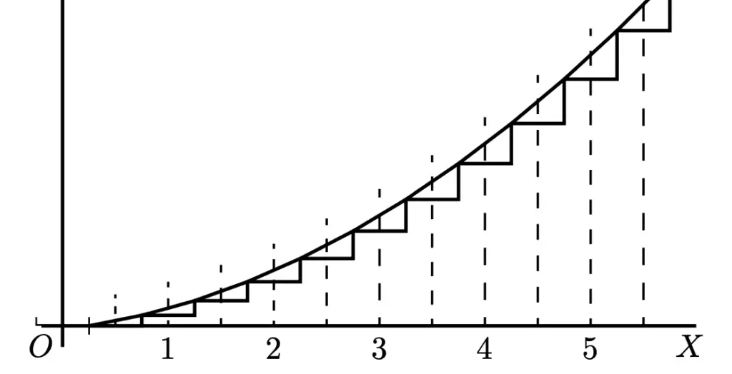
In fact, we can reduce Δx to an infinitesimally small number by using many, many rectangles, giving us an ever more accurate approximation of the area under the curve.

S = \lim_{x\to\infty}\sum_{i=1}^{n}f(x_i)Δx_i

Taking this idea ad infinity, we ultimately arrive at a continuous sum over f(x) and Δx rather than a sum of discrete values. This continuous sum F(x) gives us the area under the curve. It is expressed as an integral.

F(x) = \int f(x) Δx

Often you want to calculate the area in a certain interval between point a and another point b. So you use a definite interval. Also, remember that we originally used dx to denote an infinitesimally small value. Therefore, we’ll use dx instead of Δx.

F(x) = \int_{a}^{b} f(x) dx

The Fundamental Theorem of Calculus

Since integration is the reverse operation of differentiation, we can conclude the following.

F(x) = \int f(x) dx \\
\frac{d}{dx}F(x) = f(x)

F(x) is also referred to as the antiderivative of f(x). With this knowledge, we can rearrange and express f(x) entirely in terms of its integral and its differential.

\color{red}
f(x) = \frac{d}{dx} \int f(x) dx

This is known as the first fundamental theorem of calculus.

The second fundamental theorem of calculus states that the region under the curve f(x) within a defined interval from a to b [a,b] can be calculated by subtracting the antiderivative evaluated at b from the antiderivative evaluated at a.

\int_{a}^{b} f(x) dx = F(b) - F(a) 

I’m not going to go through the details, but if you are interested in a proof, I suggest checking out this site.

This post is part of a series on Calculus for Machine Learning. To read the other posts, go to the index.