T-Tests: A comprehensive introduction

In this post, we define the t-test in statistics, explain what different t-tests exist, and demonstrate by example how we can use them to find the differences between means in various scenarios.
What is a T-Test?
The t-test tests the significance of the difference of measured means. Differences can be measured within the same group, between groups, and against a known mean. There are paired t-tests, one-sample t-tests, and two-sample t-tests also known as independent sample t-tests.
The paired t-test is used to compare mean differences within a group. Comparisons of differences within a group are often used to measure the significance of changes over time. For example, if you are interested in the change in blood pressure of a group of people over time, you are comparing means within a group. You record the blood pressure of a group of people today and record it again in one year. Then you check whether the means differ significantly using a paired t-test.
The two-sample t-test is used to compare the mean difference between two groups. A classical example is the use of an experimental group and a control group when testing new medications. The experimental group receives the medication while the control group does not. The two-sample t-test can then be used to compare the mean difference in response measures to the medication to see whether it has a statistically significant effect.
The one-sample t-test is used to compare the mean of one group against a known or expected mean. For example, you measure the diastolic blood pressure of a group of people and compare it to the expected mean diastolic blood pressure of 70.
T Test vs Z Test
The t-test and the z-test both determine whether the measured difference between means is statistically significant. For large sample sizes of roughly more than 30 subjects, both tests should deliver almost identical results. For smaller sample sizes the t-test is more appropriate. Due to the use of degrees of freedom, the t-test is better able to account for the larger variance that comes with smaller test samples. To be on the safe side, I recommend generally using a t-test over a z-test regardless of the sample size.
If you want to learn more about the t-distribution and how it differs from the z distribution, check out this post.
One-Tailed vs Two-Tailed T-Test
One-tailed t-tests are used when you are only interested in the difference in one direction. An example would be if you are testing a blood pressure medication on an experimental group and a control group and you want to test whether the medication lowers blood pressure.
The two-sided test is appropriate when you want to determine whether there generally is a statistically significant difference between means regardless of the direction. If you don’t know the direction of your difference or want to test for the possibility of differences in both directions, you should use the two-tailed t-test.
T-Test Assumptions
When applying a t-test, the following assumptions need to be satisfied:
- Normality: The data needs to be approximately normally distributed
- Representative Sample: The sample must be representative of the population it was drawn from
- Continuous or Ordinal Scale of Measurement: The collected data must be on a continuous or ordinal scale
- Homogeneity of Variance: The variances of the samples need to be approximately equal (testing samples with different variances is possible using an adjusted t-test)
The Paired T-Test
Using the paired sample t-test we can calculate the differences between observations within a group. If you test the same people in a group twice with a difference in time or in different settings, your observations are paired.
We calculate the paired t-test statistic using the following formula.
t = \frac{X_{d} - \mu_{d}}{\frac{S_{d}}{\sqrt{n_{d0}}}}X_d is the mean difference between observations, and S_d is the standard deviation of the difference between observations. The mu_d is the expected value given the null hypothesis. Since your null hypothesis stipulates that there is no difference, this value equals 0. Let’s walk through an example to see how the formula is applied in practice.
Paired T-Test Example
Assume we have developed a novel blood pressure medication and we want to test it on a (very small) group of people for a period of two months to see whether it significantly impacts blood pressure in either direction.
We hypothesize that there is a significant difference between means.
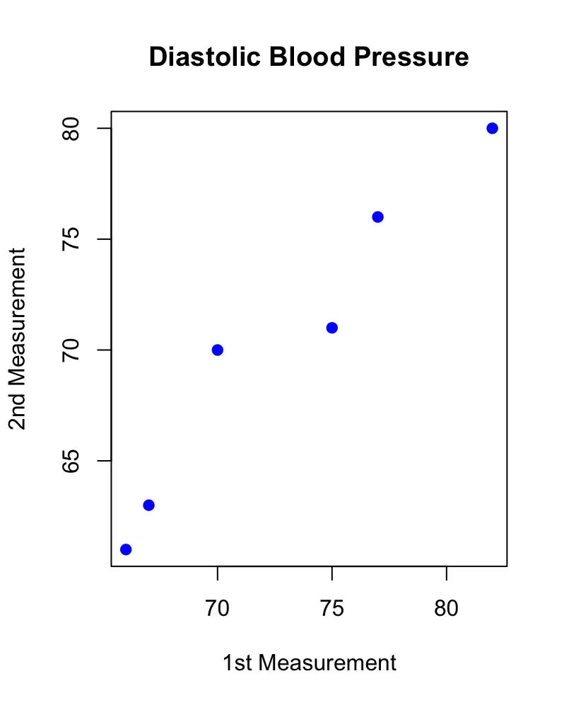
There are 6 subjects in the group whose blood pressure has been measured first before starting treatment and then after 2 months.
| Subjects | 1st Measurement | 2nd Measurement | Difference |
| 1 | 75 | 71 | 4 |
| 2 | 82 | 80 | 2 |
| 3 | 77 | 76 | 1 |
| 4 | 67 | 63 | 4 |
| 5 | 70 | 70 | 0 |
| 6 | 66 | 61 | 5 |
As we can see in the table, there are differences between the first measurement and the second measurement. Plotting the measurements against each other also reveals that there is a slight difference. If the measurements were the same, the observations would line up on the diagonal.
But are these differences statistically significant? To find out we have to calculate the mean, the standard deviation and the count of the observed differences and plug these values into the formula.
X_d = 2.66\\
S_d = 1.966 \\
n_d = 6
t = \frac{2.66 - 0}{\frac{1.966}{\sqrt{6}}}t = 3.32
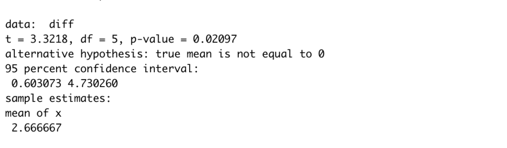
Using the statistical software R, we can easily calculate the p-value using the pt function. Here we calculate the area under the upper tail of the t distribution. Multiplying this by two gives us the 2 tailed p-value.
2* pt(abs(t), n -1, lower.tail = F) # 0.02096634
The result is statistically significant with a p-value of 0.02 if we use 0.05 as a cutoff.
Using R, we could also have used the inbuilt t.test function on the differences, which would have performed the procedure automatically, and returned the following neat result.
Two-Sample T-Test
In a two-sample t-test, you test whether the difference between two observed group means is statistically significant. This requires a different approach than when comparing subjects from the same group at different times as in the paired t-test.
The reason for choosing a different test is that results from the same subject tend to have a positive correlation. For example, a person that has had a higher than normal blood pressure on the first measurement is likely to have elevated blood pressure the second time. If a person tends to become nervous when entering a doctor’s office, it will likely affect her blood pressure on both occasions. If, on the other hand, you are comparing two measurements from different people, this correlation doesn’t exist. Your subject from the first group could be a hypochondriac with elevated blood pressure while the corresponding subject in the second group is laid back and relaxed and has completely normal blood pressure.
A two-sample -test is calculated according to the following formula:
t = \frac{X_1 - X_2}{S_p\sqrt{\frac{1}{n_1} + \frac{1}{n_2}}}where X_1 and X_2 are the means of the observations from the first and the second group, S_p represents the pooled standard deviation, and n_1 and n_2 are the numbers of observations in the X_1 and X_2 respectively.
Two-Sample T-Test Example
Suppose we have two groups. One of them is following a special diet. The second one is not. We want to figure out whether the diet has a statistically significant effect on diastolic blood pressure.
Our hypothesis is that the diet does not affect diastolic blood pressure.
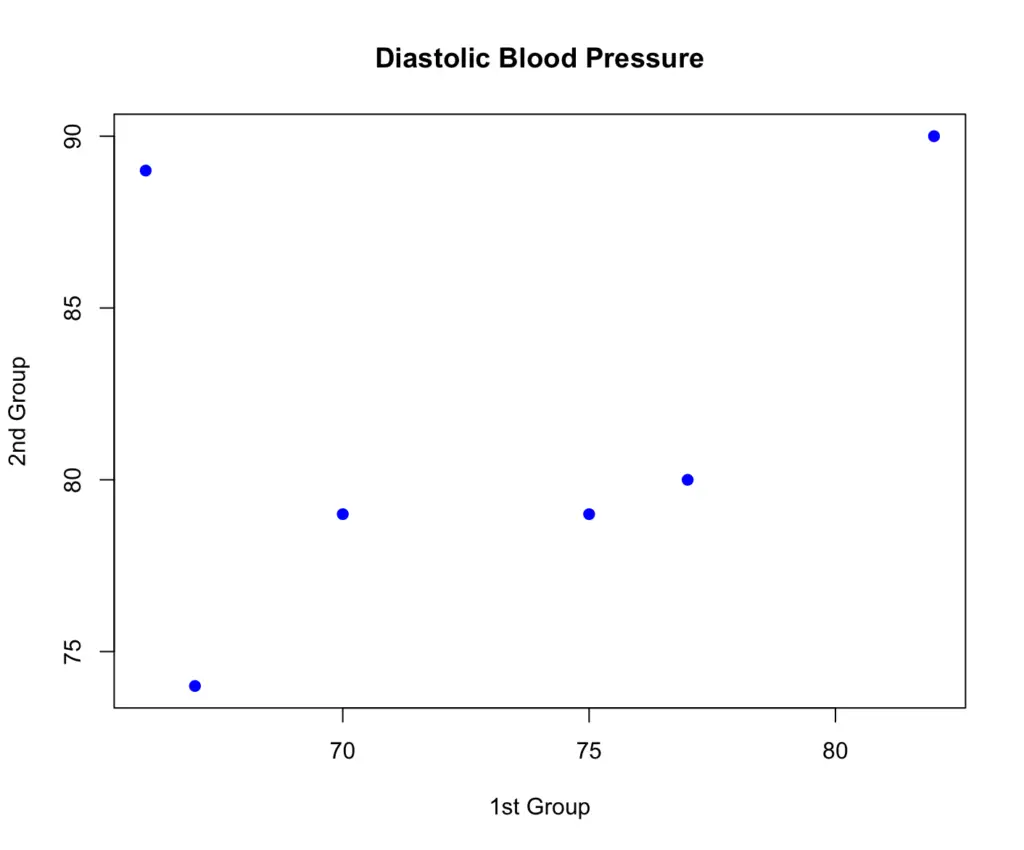
| Subjects | 1st Group (Special Diet) | 2nd Group (No Special Diet) |
| 1 | 75 | 79 |
| 2 | 82 | 90 |
| 3 | 77 | 80 |
| 4 | 67 | 74 |
| 5 | 70 | 79 |
| 6 | 66 | 89 |
When plotting the first group against the second, there appears to be a difference between the two groups in terms of blood pressure measurements.
To figure out whether the difference is statistically significant, we need to plug the values into our formula for the two-sided t-test. First, we have to obtain the means and the counts of the two groups. This is relatively straightforward, so I’ll skip the calculation.
X_1 = 72.8 \\
X_2 = 81.8\\
n_1 = 6\\
n_2 = 6
Next, we need to calculate the pooled variance of the two groups according to the following formula:
S_p^2 = \frac{(n_1 - 1)S_1^2 + (n_2 - 1)S_2^2}{(n_1 + n_2) -2}To obtain the pooled standard deviation, we take the square root of the pooled variance.
S_p = \sqrt{S_p^2}Plugging our values into this formula gives us a pooled standard deviation of 6.27.
S_p = 6.27
Now we are ready to calculate the t statistic.
t = \frac{72.8 - 81.8}{6.27\sqrt{\frac{1}{6} + \frac{1}{6}}} = -2.48Using R, we calculate the p-value, which turns out to be roughly 0.03. So we can reject the null hypothesis. Seems like the diet does have an effect on blood pressure.
2 * pt(abs(t), 10, lower.tail = F) # 0.03229305
Note that the degrees of freedom are 10 because we have two samples of size 6. We deduct one from each and add them up to obtain the degrees of freedom.
One-Sample T-Test
The one sample t-test is simpler than the preceding ones because you only need to compare one group against an already established expected mean. You do this according to the classic t-test formula.
t = \frac{X - \mu}{\frac{s}{\sqrt{n}}}Where X is the mean of the sample, mu is the expected mean, s is the group standard deviation, and n is the number of observations within the group.
One-Sample T-Test Example
Let’s return to our example concerning diastolic blood pressure. This time our null hypothesis is that the mean blood pressure of the group does not deviate significantly from the expected mean of 70. In other words, we expect the mean systolic blood pressure to equal 70.
| Subjects | Group |
| 1 | 75 |
| 2 | 82 |
| 3 | 77 |
| 4 | 67 |
| 5 | 70 |
| 6 | 66 |
We calculate the group mean, standard deviation and count which results in the following values.
X = 72.8 \\
s = 6.24 \\
n = 6
Next, we plug these values into our formula.
t = \frac{72.8 - 70}{\frac{6.24}{\sqrt{6}}} = 1.1118Using R, we calculate the p-value, which tells us that we do not have enough evidence to reject the null hypothesis at the 5% significance level.
2 * pt(abs(t), 5, lower.tail = F) # 0.3168


