Identity Matrix and Inverse Matrix

We introduce the inverse matrix and the identity matrix. In addition, we learn how to solve systems of linear equations using the inverse matrix.

The identity matrix is a matrix in which the diagonal entries are 1, and all other entries are zero. It is a more restrictive form of the diagonal matrix.

I =   \begin{bmatrix}
    1 & 0 & 0 \\
    0 & 1 & 0 \\
    0 & 0 & 1 \\

  \end{bmatrix}

It is the matrix equivalent to 1 for real numbers. This means multiplying a matrix A by the identity matrix produces A.

A I = A    

As long as the dimensions match, you could also write this as 

IA = A

For example:

  \begin{bmatrix}
    1 & 0 \\
    0 & 1  \\


  \end{bmatrix}

  \begin{bmatrix}
    1 & 3  \\
    2 & 4  \\


  \end{bmatrix}

=
  \begin{bmatrix}
    1 & 3  \\
    2 & 4  \\


  \end{bmatrix}

  \begin{bmatrix}
    1 & 0 \\
    0 & 1  \\


  \end{bmatrix}
=
  \begin{bmatrix}
    1 & 3  \\
    2 & 4  \\


  \end{bmatrix}

Inverse Matrix

The inverse matrix is closely related to the identity matrix. Multiplying a matrix by its inverse always yields the identity matrix.

AA^{-1} = I

For example:

  \begin{bmatrix}
    3 & 2  \\
    4 & 3  \\


  \end{bmatrix}


  \begin{bmatrix}
    3 & -2  \\
    -4 & 3  \\


  \end{bmatrix}


=
  \begin{bmatrix}
    1 & 0  \\
    0 & 1  \\


  \end{bmatrix}

Note that not every matrix has an identity matrix.

Solving Linear Systems with the Inverse Matrix

We’ve established that a linear system of equations can be represented as a matrix of coefficients A multiplied by a vector b of your unknown variables, to give you the vector of results c.

Ab = c

Using Gaussian elimination we can determine the values of b. But this only gives you a solution for a specific value of c. If c changes, you’d have to do the whole process of Gaussian elimination all over again.

Imagine you have a car production plant for trucks and cars and your production target is 10 trucks and 8 cars.
You need 1 unit of materialA and 3 units of materialB to produce a certain amount of trucks and 1 unit of materialA and 2 units of materialB to produce cars.

Assume also that the production lines are interdependent. For example changes in the production of cars could affect units of materials required for truck production because trucks make us of preprocessed materials from the car production line, etc.

You could model this with our Ab = c  format and figure out the solution using Gaussian elimination:

  \begin{bmatrix}
    1 & 3 \\
    1 & 2 \\
  \end{bmatrix}


  \begin{bmatrix}
    materialsA \\
    materialsB \\
  \end{bmatrix}
 =

  \begin{bmatrix}
    10 \\
    8 \\
  \end{bmatrix}

With Gaussian elimination the solution is materialsA = 4 and materialsB = 2.

Your production targets are likely to change. For this small example it is not a big deal. But in the real world you rarely deal with such small examples. In data science and machine learning you often have millions of dimensions in your vectors and matrices.

Applying Gauss Jordan elimination across all these dimensions for every change is highly inefficient.

Luckily, this can be avoided with the help of the identity matrix and the inverse matrix.

Starting from your original form

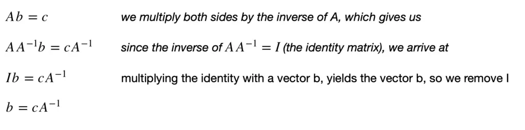
If our production targets c change, now all we have to do is multiply the new c with the inverse of A to get to our new b values.

We can now apply Gauss Jordan elimination to find the identity of a matrix.

AA^{-1} = I

Unfortunately we cannot divide by matrices, so we cannot say

\color{red}
A^{-1} = \frac{I}{A} \, = wrong!

But what we can do instead is turn A into I by Gaussian elimination. Then we have IA^{-1} on the left side, which is equivalent to A^{-1}, and our solution remains on the right.

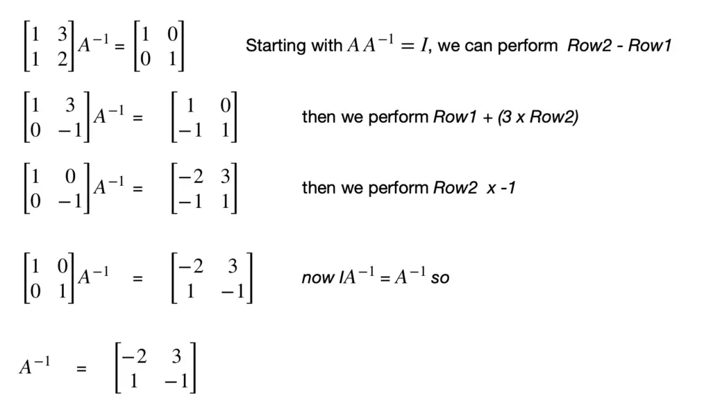
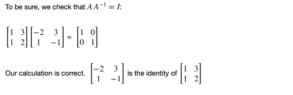
Let’s plug this into our car production plant example (we used the same coefficient matrix A).

We concluded that for

  \begin{bmatrix}
    1 & 3 \\
    1 & 2 \\
  \end{bmatrix}


  \begin{bmatrix}
    materiala \\
    materialb \\
  \end{bmatrix}
=

  \begin{bmatrix}
    10 \\
    8 \\
  \end{bmatrix}

Let’s multiply our result vector c with the inverse matrix of A to get b. It should give us the same result

  \begin{bmatrix}
    10 \\
    8 \\
  \end{bmatrix}


  \begin{bmatrix}
    -2 & 3 \\
    1 & -1 \\
  \end{bmatrix}

=
  \begin{bmatrix}
    materialsA \\
    materialsB \\
  \end{bmatrix}
=
  \begin{bmatrix}
    4 \\
    2 \\
  \end{bmatrix}

Indeed, it does give us the expected result.

This post is part of a series on linear algebra for machine learning. To read other posts in this series, go to the index.