Geometric Distribution and Geometric Random Variables

In this post we introduce the geometric distribution with an example and discuss how to calculate the probability of geometric random variables.

The geometric distribution describes the probability of the number of failures before a successful outcome in a Bernoulli trial.

Suppose you are a recruiter and you need to find a suitable candidate to fill an IT job. Unfortunately for you, great IT talent is hard to come by, and your chance that a suitable candidate will be interested is 15%. Using the geometric distribution, you could calculate the probability of finding a suitable candidate after a certain number of failures.

Geometric Distribution Formula

Like the Bernoulli and Binomial distributions, the geometric distribution has a single parameter p. the probability of success.

P(X=x) = (1-p) ^{x-1} p

The mean and variance of a geometric random variable can be calculated as follows:

\mu = \frac{1}{p} \;\;\;\; and \;\;\;\sigma^2 = \frac{1-p}{p^2}

Let’s go back to our recruiting scenario and calculate the probability of finding a suitable candidate on the third attempt. We just plug the numbers into the formula.

P(X=3) = (1-0.15)^{(3-1)}0.15 = 0.108

As you can see in the following plot, the probability of getting the right candidate declines on each successive attempt.

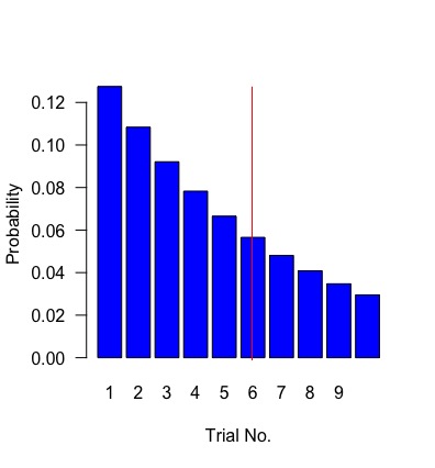
This makes sense since it is more probable that we already found a suitable candidate in one of the preceding trials. As a recruiter rather than knowing whether you’ll find a candidate on a specific trial, you are probably more interested in the cumulative probability of finding a candidate after a certain number of trials. If you message three candidates, you probably don’t care whether the first or the third one answers positively (I’m ignoring preferences based on the candidates’ individual qualifications). You only care that you find at least one candidate who answers.

We can model this situation using the cumulative geometric distribution.

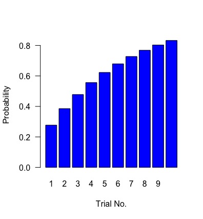
To calculate the cumulative distribution function, you just add up all the preceding probabilities.

P(X \leq 3) = P(X=1) + P(X=2) + P(X=3) = 0.48

Your chances of having at least one candidate who replies positively stand at almost 50%

The mean and variance resolve to the following values.

\mu = \frac{1}{0.15} = 6.66

\sigma^2 = \frac{1-0.15}{0.15^2} = 37.78

If these values seem unusually large, you have to consider that the geometric distribution has no upper bound. Theoretically, you could message an infinite number of candidates without ever getting a positive reply. The probability that this happens is infinitesimally small. But the mere possibility of an infinite number of trials increases the variance significantly and pulls the mean upwards.

This post is part of a series on statistics for machine learning and data science. To read other posts in this series, go to the index.