What is a Diagonal Matrix

We introduce and discuss the applications and properties of the diagonal matrix, the upper triangular matrix, and the lower triangular matrix.
A diagonal matrix is a square matrix in which all entries are zero, except for those on the leading diagonal. It is also called the scaling matrix because multiplication with the diagonal matrix scales an object in a corresponding vector space.
The following matrices may be confused as diagonal matrices. They are not diagonal because they do not have the square form.
   \begin{bmatrix}
    1 & 0   \\
    0 & 3   \\
    0 & 0  \\

  \end{bmatrix} \;\;

   \begin{bmatrix}
    0 & 0   \\
    1 & 0   \\
    0 & 3  \\

  \end{bmatrix}
\;\;
   \begin{bmatrix}
    1 & 0 & 0  \\
    0 & 3 & 0  \\
  \end{bmatrix}
The following matrix, on the other hand, is diagonal. The fact that some entries along the diagonal are zero is irrelevant.
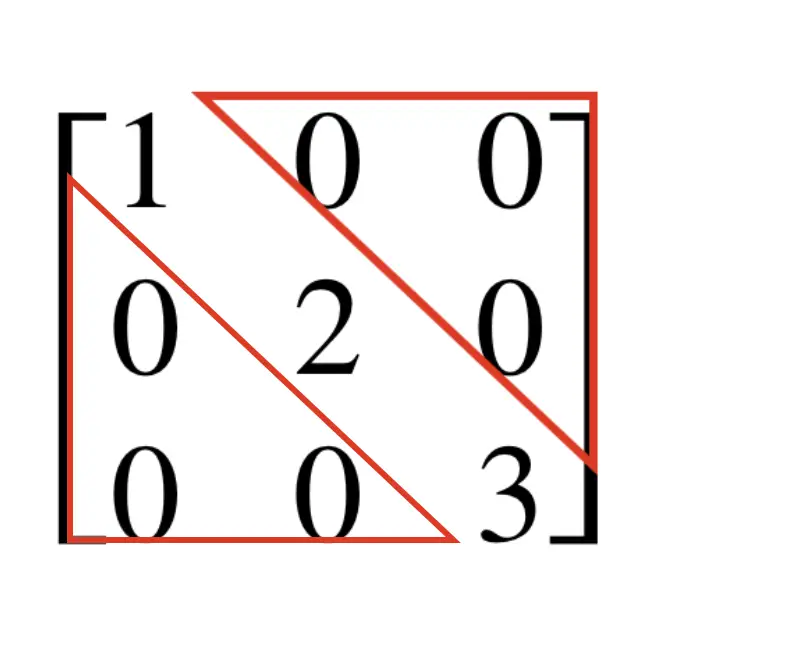
   \begin{bmatrix}
    1 & 0 & 0  \\
    0 & 0 & 0  \\
    0 & 0 & 6  \\

  \end{bmatrix}
A diagonal matrix also has the properties of an upper triangular matrix and a lower triangular matrix.
Upper Triangular Matrix
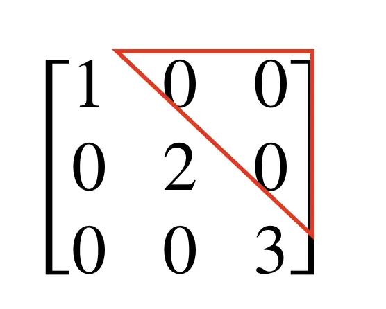
An upper triangular matrix consists out of zero entries below the main diagonal.
An upper triangular matrix is not necessarily a diagonal matrix. The following matrix is upper triangular, but not diagonal.
   \begin{bmatrix}
    1 & 2 & 3  \\
    0 & 4 & 5  \\
    0 & 0 & 6  \\

  \end{bmatrix}
Lower Triangular Matrix
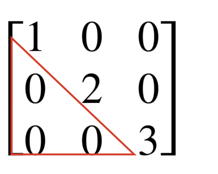
In an lower diagonal matrix, only the entries above the main diagonal have to be zero.
A lower triangular matrix is also not necessarily a diagonal matrix. Here is an example of a lower triangular matrix that is not diagonal.
   \begin{bmatrix}
    1 & 0 & 0  \\
    2 & 3 & 0  \\
    4 & 5 & 6  \\

  \end{bmatrix}
What’s the use of diagonal and triangular matrices
If the entries below the diagonal are zero, the matrix is in row echelon form. This implies, that the linear system defined by the matrix can easily be solved through substitution. Gauss Jordan elimination is not necessary.
Note, that you can easily transform an upper triangular matrix into row echelon form by rearranging the rows.
Backward Substitution with an Upper Triangular Matrix
Assume we have a set of equations in the form
Ax = b
With an upper triangular matrix, the full matrix is of the following form.
   \begin{bmatrix}
    a_{11} & ... & a_{1. n-1} & a_{1. n}    \\
    ... & ... & ... & ... & \\
   0 & ... & a_{n-1. n-1} & a_{n-1. n} \\
    0 & 0 & 0 & a_{n, n}   \\
  \end{bmatrix}

 \begin{bmatrix}
x_1 \\
...\\
x_{n-1} \\
x_n
\end{bmatrix}

=
\begin{bmatrix}
b_1 \\
...\\
b_{n-1} \\
b_n
\end{bmatrix}
This means the system can be resolved by backward substituting the equations.
Let’s do an example to make this clearer.
  \begin{bmatrix}
1 & 2& 1 \\
0 & 1& 3 \\
0 & 0& 2 \\
  \end{bmatrix}
\begin{bmatrix}
x \\
y \\
z
  \end{bmatrix}
=
\begin{bmatrix}
0 \\
1 \\
2
  \end{bmatrix}
This results in the following equations:
x+2y+z =0 \\
y+3z = 1 \\
2z = 2
The system can be resolved by a procedure known as backward substitution, where we start with resolving the last equation and substituting the results in the equations above.
z = 1 \\
y = 1 - 3 z = 2 \\
x = 0 -2y -z =-5
Forward Substitution with a Lower Triangular Matrix
We start again with an equation of the basic form.
Ax = b
This time, the area above the diagonal in A consists of zeros.
   \begin{bmatrix}
    a_{11} & 0 & ... & 0   \\
    a_{21} & a_{22} & ... & 0 & \\
   ... & ... & ... & ... \\
    a_{n, 1} & a_{n, 2} & ... & a_{n, n}   \\
  \end{bmatrix}

 \begin{bmatrix}
x_1 \\
...\\
x_{n-1} \\
x_n
\end{bmatrix}

=
\begin{bmatrix}
b_1 \\
...\\
b_{n-1} \\
b_n
\end{bmatrix}
Let’s consider the following example:
  \begin{bmatrix}
1 & 0& 0 \\
2 & 3& 0 \\
1 & 1& 1\\
  \end{bmatrix}
\begin{bmatrix}
x \\
y \\
z
  \end{bmatrix}
=
\begin{bmatrix}
1 \\
5 \\
3
  \end{bmatrix}
The individual equations look like this:
x = 1 \\
2x + 3y = 5 \\
x+y+z = 3
Now we can forward substitute the values starting with the first equation and working our way down.
x = 1\\
y = (5 - 2x ) / 3 = 1 \\
z = 3 -x -y = 3
Properties of a Diagonal Matrix
Diagonal Matrix Multiplication
If we multiply any matrix A with a diagonal matrix D, the multiplication becomes easier since we don’t have to perform the full dot product.
If you perform AD, then all you need to do is multiply every column in A with the non-zero diagonal element in the same column in D:
   \begin{bmatrix}
    1 & 3  \\
    2 & 4  \\

  \end{bmatrix}

 \begin{bmatrix}
    1 & 0 \\
    0 & 2  \\

  \end{bmatrix}

=
 \begin{bmatrix}
    1 & 6 \\
    2 & 8  \\

  \end{bmatrix}
If you perform DA, then all you need to do is multiply every row in A with the non-zero diagonal element in the same row in D:
   \begin{bmatrix}
    1 & 0 \\
    0 & 2  \\

  \end{bmatrix}

 \begin{bmatrix}
    1 & 3  \\
    2 & 4  \\

  \end{bmatrix}

=
 \begin{bmatrix}
    1 & 3 \\
    4 & 8  \\

  \end{bmatrix}
In vector space this results in scaling the object along the dimensions of the corresponding diagonal.
If you multiply two diagonal matrices, they need to be of the same order. The result will again be a diagonal matrix.
 \begin{bmatrix}
    1 & 0 \\
    0 & 2  \\

  \end{bmatrix}


 \begin{bmatrix}
    4 & 0 \\
    0 & 6  \\

  \end{bmatrix} =

 \begin{bmatrix}
    4 & 0 \\
    0 & 12  \\

  \end{bmatrix}
Diagonal Matrix Addition
Matrix addition can be performed between two matrices of the same order. The result will again be a diagonal matrix.
   \begin{bmatrix}
    2 & 0  \\
    0 & 4  \\
  \end{bmatrix}
+
   \begin{bmatrix}
    6 & 0  \\
    0 & 8  \\
  \end{bmatrix}
=

 \begin{bmatrix}
    8 & 0 \\
    0 & 12  \\

  \end{bmatrix}
Transpose of a Diagonal Matrix
The transpose of a diagonal matrix is equivalent to the diagonal matrix.
A^T = A
For example:
A =    \begin{bmatrix}
    2 & 0  \\
    0 & 4  \\
  \end{bmatrix}
\;
A^T =    \begin{bmatrix}
    2 & 0  \\
    0 & 4  \\
  \end{bmatrix}
Inverse of a Diagonal Matrix
The inverse diagonal matrix contains the reciprocal values of the diagonal matrix.
A = \begin{bmatrix}
    2 & 0  \\
    0 & 4  \\
  \end{bmatrix}
\;
A^{-1} =
\begin{bmatrix}
    1/2 & 0  \\
    0 & 1/4  \\
  \end{bmatrix}
Determinant of a Diagonal Matrix
The determinant of a diagonal matrix equals the product of all values along the diagonal in the matrix.
A = \begin{bmatrix}
    2 & 0  \\
    0 & 4  \\
  \end{bmatrix}
\;
det(A) =  8
Summary
This post is part of a series on linear algebra for machine learning. To read other posts in this series, go to the index.
