Factorization Theorem and the Exponential Family
In this post we introduce Fisher’s factorization theorem and the concept of sufficient statistics. We learn how to use these concepts to construct a general expression for various common distributions known as the exponential family.
In applied statistics and machine learning we rarely have the fortune of dealing with a known distribution with known parameters. We’ve already discussed maximum likelihood estimation as a method to estimate unknown parameters of a known or assumed distribution.
We can raise the level of abstraction, even more, by considering families of distributions. The exponential family, which includes distributions such as the Gaussian and the Bernoulli, is particularly useful. To describe it, we first need to introduce the factorization theorem and the concept of sufficient statistics.
Sufficient Statistic
In the preceding posts, we’ve discussed probability and statistics. But until now, we haven’t introduced a formal definition of statistics yet.
A statistic is a function of a random variable.
For example, the mean \tilde\mu of a normally distributed data sample x can be calculated from the data points using the following function.
\tilde\mu = \frac{1}{n} (x_1, x_2, ...,x_n)We say that the sample mean is a statistic of the random variable X.
A statistic is sufficient if no more information about the true distribution parameters can be inferred from the given sample.
For example, the mean of the data sample x for a normally distributed random variable with known variance is a sufficient statistic. You do not need to know all the data that defines the distribution. The sample is enough to estimate the true mean.
Factorization Theorem
The concept of sufficient statistics is formalized in Fisher’s factorization theorem.
Assume you have a random variable X with distribution parameterized by an unknown parameter θ.
f(x|\theta)
Note: capital X is the random variable, while x is the set of concrete realized values that the variable assumes.
Since we don’t know θ, we would like to find a way to describe the distribution over X without θ.
To achieve this goal, we obtain a statistic t(x) from a subsample of x that characterizes θ. If t(x) is a sufficient statistic, it should encapsulate all the necessary knowledge about θ. Accordingly, it should be possible to describe the distribution over X without θ by factoring it into a component h(x) that does not depend on θ and one component g(t(x)) that can be sufficiently explained by our sample statistic t(x).
f(x|\theta) = h(x)g(t(x))
Exponential Family
Using the sufficient statistic, we can construct a general form to describe distributions of the exponential family.
f(x|\theta) = h(x)exp(\theta \cdot t(x) -A(\theta))
You calculate the dot product between the vector of unknown parameters θ and the vector of sufficient statistics. Then you subtract the normalization term A(θ), take the exponent of the whole expression, and multiply it by the part h(x) that does not depend on θ.
Note: Mathematically, the normalization term A(θ) ensures that the expression integrates to 1, which is a requirement of probability density functions in general, or sums to 1 in the case of probability mass functions.
This is very abstract, so let’s have a look at a concrete distribution to show why it is part of the exponential family.
The Gaussian as Part of the Exponential Family
The Gaussian has the following probability density function parameterized by its mean, and standard deviation.
f(x|\mu, \sigma^2) = \frac{1}{\sqrt{2\pi\sigma^2}} exp(\frac{(x-\mu)^2}{2\sigma^2})Let’s multiply the term inside the exponential out.
f(x|\mu, \sigma^2) = \frac{1}{\sqrt{2\pi\sigma^2}}
exp(\frac{x^2}{2\sigma^2} - \frac{2x\mu}{2\sigma^2} + \frac{\mu^2}{2\sigma^2})
and bring \sigma^2 out of the denominator and into the exponential term by taking its negative log. I’ve also algebraically reorganized the terms inside the exponential a bit.
f(x|\mu, \sigma^2) = \frac{1}{\sqrt{2\pi}}
exp(  \frac{x\mu}{\sigma^2} - \frac{x^2}{2\sigma^2} - \frac{\mu^2}{2\sigma^2} -log(\sigma))
Now, our normal resembles the general exponential form. We can simply pick out the constituent parts.
The parameter-independent part:
h(x) = \frac{1}{\sqrt{2\pi}} Our vector of sufficient statistics:
t(x) = [x, x^2]
Our parameter vector θ:
\theta = [\frac{\mu}{\sigma^2}, \frac{-1}{2\sigma^2}]^TThe normalization term A(θ):
A(\theta) = \frac{\mu^2}{2\sigma^2}-log(\theta)The Binomial as Part of the Exponential Family
We’ve previously introduced the Bernoulli distribution which can be written as a conditional probability of the realized outcome x given the probability of an outcome p.
f(x|p) = p^x(1-p)^{1-x}Let’s go try to bring this into our characteristic exponential family-form. We start by moving everything into an exponential. To retain equivalency to the original form, we have to apply the natural logarithm which reverses the exponential operation.
p(x|p) = exp(log(p^x(1-p)^{1-x}))Remember, that the logarithm reduces powers to multiplications and multiplications to additions. We can, thus, gradually move parts of our expression out of the log.
p(x|p) = exp(x \log(p) + (1-x) \ log(1-p)))
p(x|p) = exp(x \log(p) + 1 \ log(1-p) - x \ log(1-p) ))
p(x|p) = exp(x \ \log(\frac{p}{1-p}) + log(1-p) ))We’ve arrived at our characteristic exponential family form and we can pluck out the parameters.
h(x) =1
\theta = log(\frac{p}{1-p})t(x) = x
A(\theta) = -log(1-p)
For machine learning applications, it is especially interesting that the relationship between θ and p is invertible because it allows us to construct the sigmoid function.
p = \frac{1}{1+exp(-\theta)}This is a commonly used activation function in neural networks.
Wrap Up
We’ve introduced the exponential family and its constituting parts by learning about Fisher’s factorization theorem and the concept of the sufficient statistic.
Understanding maximum likelihood, the general form of the exponential family, and its most important distributions is a strong building block in our mathematical foundation for machine learning and data science.
This post is part of a series on statistics for machine learning and data science. To read other posts in this series, go to the index.


