Maximum Likelihood Estimation Explained by Example

In this post, we learn how to calculate the likelihood and discuss how it differs from probability. We then introduce maximum likelihood estimation and explore why the log-likelihood is often the more sensible choice in practical applications.

Maximum likelihood estimation is an important concept in statistics and machine learning. Before diving into the specifics, let’s first understand what likelihood means in the context of probability and statistics

Probability vs Likelihood

You can estimate a probability of an event using the function that describes the probability distribution and its parameters. For example, you can estimate the outcome of a fair coin flip by using the Bernoulli distribution and the probability of success 0.5. In this ideal case, you already know how the data is distributed.

But the real world is messy. Often you don’t know the exact parameter values, and you may not even know the probability distribution that describes your specific use case. Instead, you have to estimate the function and its parameters from the data. The likelihood describes the relative evidence that the data has a particular distribution and its associated parameters.

We can describe the likelihood as a function of an observed value of the data x, and the distributions’ unknown parameter θ.

f(x,\theta)

In short, when estimating the probability, you go from a distribution and its parameters to the event.

Probability: p(event|distribution)

When estimating the likelihood, you go from the data to the distribution and its parameters.

Likelihood: L(distribution|data)

To make this more concrete, let’s calculate the likelihood for a coin flip.

Recall that a coin flip is a Bernoulli trial, which can be described in the following function.

P(X = x) = p^x(1-p)^{1-x}

The probability p is a parameter of the function. To be consistent with the likelihood notation, we write down the formula for the likelihood function with theta instead of p.

L(x, \theta) = \theta^x(1-\theta)^{1-x}

Now, we need a hypothesis about the parameter theta. We assume that the coin is fair. The probability of obtaining heads is 0.5. This is our hypothesis A.

Let’s say we throw the coin 3 times. It comes up heads the first 2 times. The last time it comes up tails. What is the likelihood that hypothesis A given the data?

First, we can calculate the relative likelihood that hypothesis A is true and the coin is fair. We plug our parameters and our outcomes into our probability function.

P(X = 1) = 0.5^1(1-0.5)^{1-0} = 0.5

P(X = 1) = 0.5^1(1-0.5)^{1-0} = 0.5

P(X = 0) = 0.5^0(1-0.5)^{1-0} = 0.5

Multiplying all of these gives us the following value.

\frac{1}{2} \times \frac{1}{2} \times \frac{1}{2} = \frac{1}{8}

Likelihood Ratios

Once you’ve calculated the likelihood, you have a hypothesis that your data has a specific set of parameters. The likelihood is your evidence for that hypothesis. To pick the hypothesis with the maximum likelihood, you have to compare your hypothesis to another by calculating the likelihood ratios.

Since your 3 coin tosses yielded two heads and one tail, you hypothesize that the probability of getting heads is actually 2/3. This is your hypothesis B

Let’s repeat the previous calculations for B with a probability of 2/3 for the same three coin tosses. I won’t go through the steps of plugging the values into the formula again.

\frac{2}{3} \times \frac{2}{3} \times \frac{1}{3} = \frac{4}{27}

Given the evidence, hypothesis B seems more likely than hypothesis A.

In other words: Given the fact that 2 of our three coin tosses landed up heads, it seems more likely that the true probability of getting heads is 2/3. In fact, in the absence of more data in the form of coin tosses, 2/3 is the most likely candidate for our true parameter value. So hypothesis B gives us the maximum likelihood value.

We can express the relative likelihood of an outcome as a ratio of the likelihood for our chosen parameter value θ to the maximum likelihood.

The relative likelihood that the coin is fair can be expressed as a ratio of the likelihood that the true probability is 1/2 against the maximum likelihood that the probability is 2/3.

\frac{\frac{1}{8}}{\frac{4}{27}} = 0.84

The maximum value division helps to normalize the likelihood to a scale with 1 as its maximum likelihood. We can plot the different parameter values against their relative likelihoods given the current data.

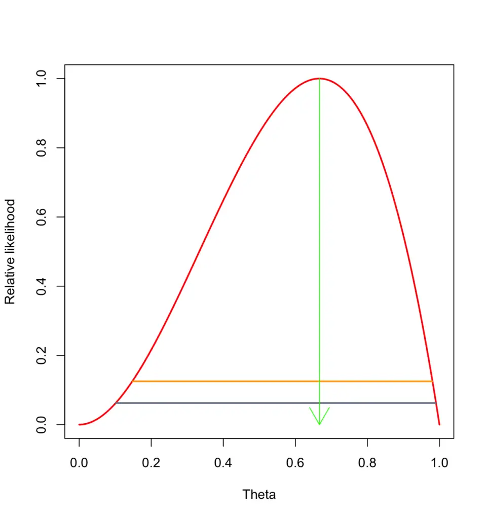
For three coin tosses with 2 heads, the plot would look like this with the likelihood maximized at 2/3.

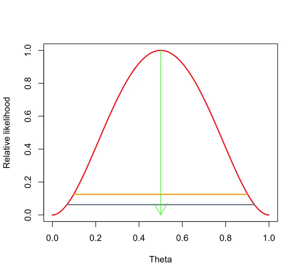
What happens if we toss the coin for the fourth time and it comes up tails. Now we’ve had 2 heads and 2 tails. Our likelihood plot now looks like this, with the likelihood maximized at 1/2.

Mathematically we can denote the maximum likelihood estimation as a function that results in the theta maximizing the likelihood.

\theta_{ML} = argmax_\theta L(\theta, x) = \prod_{i=1}^np(x_i,\theta)

The variable x represents the range of examples drawn from the unknown data distribution, which we would like to approximate and n the number of examples.

Log-Likelihood

For most practical applications, maximizing the log-likelihood is often a better choice because the logarithm reduced operations by one level. Multiplications become additions; powers become multiplications, etc.

\theta_{ML} = argmax_\theta l(\theta, x) = \sum_{i=1}^n log(p(x_i,\theta))

In computer-based implementations, this reduces the risk of numerical underflow and generally makes the calculations simpler. Since logarithms are monotonically increasing, increasing the log-likelihood is equivalent to maximizing the likelihood.

We distinguish the function for the log-likelihood from that of the likelihood using lowercase l instead of capital L.

The log likelihood for n coin flips can be expressed in this formula.

l( \theta, x) = log(\theta)x + log(1-\theta)(1-x)

Summary

The likelihood is especially important if you take a Bayesian view of the world. From a Bayesian perspective, almost nothing happens independently. Instead, events are always influenced by their environment. Accordingly, you can rarely say for sure that data follows a certain distribution. Even our fair coin flip may not be completely fair. The makeup of the coin or the way you throw it may nudge the coin flip towards a certain outcome. So, strictly speaking, before you can calculate the probability that your coin flip has an outcome according to the Bernoulli distribution with a certain probability, you have to estimate the likelihood that the flip really has that probability.

This post is part of a series on statistics for machine learning and data science. To read other posts in this series, go to the index.